Red Hat Customer Value Model
Estimated reading time: 41 minutesCredit Card Fraud Model
import numpy as np # linear algebra
import pandas as pd # data processing, CSV file I/O (e.g. pd.read_csv)
import matplotlib.pyplot as plt
%matplotlib inline
train = pd.read_csv('act_train.csv', parse_dates=['date'])
test = pd.read_csv('act_test.csv', parse_dates=['date'])
ppl = pd.read_csv('people.csv', parse_dates=['date'])

df_train = pd.merge(train, ppl, on='people_id')
df_test = pd.merge(test, ppl, on='people_id')
del train, test, ppl
First just so we know what we’re dealing with, let’s take a look at the range of the two date variables
for d in ['date_x', 'date_y']:
    print('Start of ' + d + ': ' + str(df_train[d].min().date()))
    print('  End of ' + d + ': ' + str(df_train[d].max().date()))
    print('Range of ' + d + ': ' + str(df_train[d].max() - df_train[d].min()) + '\n')
Start of date_x: 2022-07-17
  End of date_x: 2023-08-31
Range of date_x: 410 days 00:00:00

Start of date_y: 2020-05-18
  End of date_y: 2023-08-31
Range of date_y: 1200 days 00:00:00
So we can see that all the dates are a few years in the future, all the way until 2023! Although we now though that this is because the data was anonymised, so we can essentially treat these as if they were the last few years instead. We can also see that date_x is on the order of 1 year, while date_y is 3 times longer, even though they both end on the same day (the date before they stopped collecting the dataset perhaps?) We’ll go on more into looking at how the two features relate to each other later, but first let’s look at the structure of the features separately. Feature structure Here I’m grouping the activities by date, and then for each date working out the number of activities that happened on that day as well as the probability of class 1 on that day.
date_x = pd.DataFrame()
date_x['Class probability'] = df_train.groupby('date_x')['outcome'].mean()
date_x['Frequency'] = df_train.groupby('date_x')['outcome'].size()
date_x.plot(secondary_y='Frequency', figsize=(20, 10))
<matplotlib.axes._subplots.AxesSubplot at 0x7f6f58b44e10>

This plot shows some very interesting findings. There appears to be a very apparent weekly pattern, where on weekends there are much less events, as well as the probability of a event being a ‘1’ class being much lower. We can see that during the week the classes are pretty balanced at ~0.5 while on weekends they drop to 0.4-0.3 (this could be very useful information). We can also see some very big peaks in number of activities around the September-October time frame, which we will look into later in the EDA. But first, let’s do the same with the other date feature, date_y!
date_y = pd.DataFrame()
date_y['Class probability'] = df_train.groupby('date_y')['outcome'].mean()
date_y['Frequency'] = df_train.groupby('date_y')['outcome'].size()
# We need to split it into multiple graphs since the time-scale is too long to show well on one graph
i = int(len(date_y) / 3)
date_y[:i].plot(secondary_y='Frequency', figsize=(20, 5), title='date_y Year 1')
date_y[i:2*i].plot(secondary_y='Frequency', figsize=(20, 5), title='date_y Year 2')
date_y[2*i:].plot(secondary_y='Frequency', figsize=(20, 5), title='date_y Year 3')
<matplotlib.axes._subplots.AxesSubplot at 0x7f6f58d742e8>
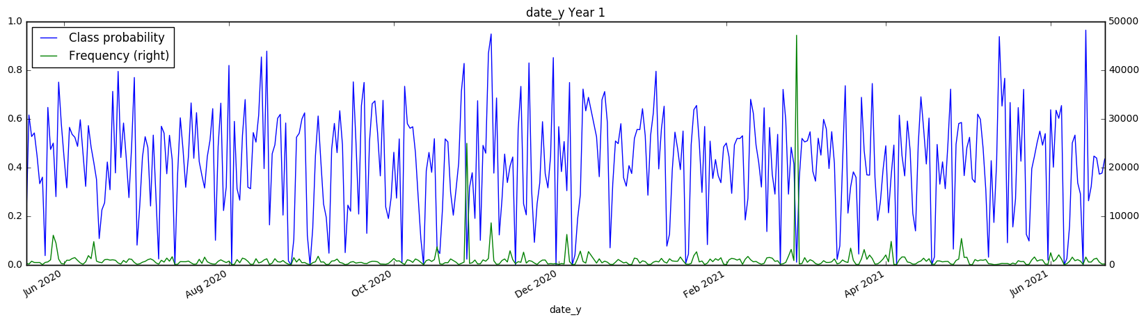
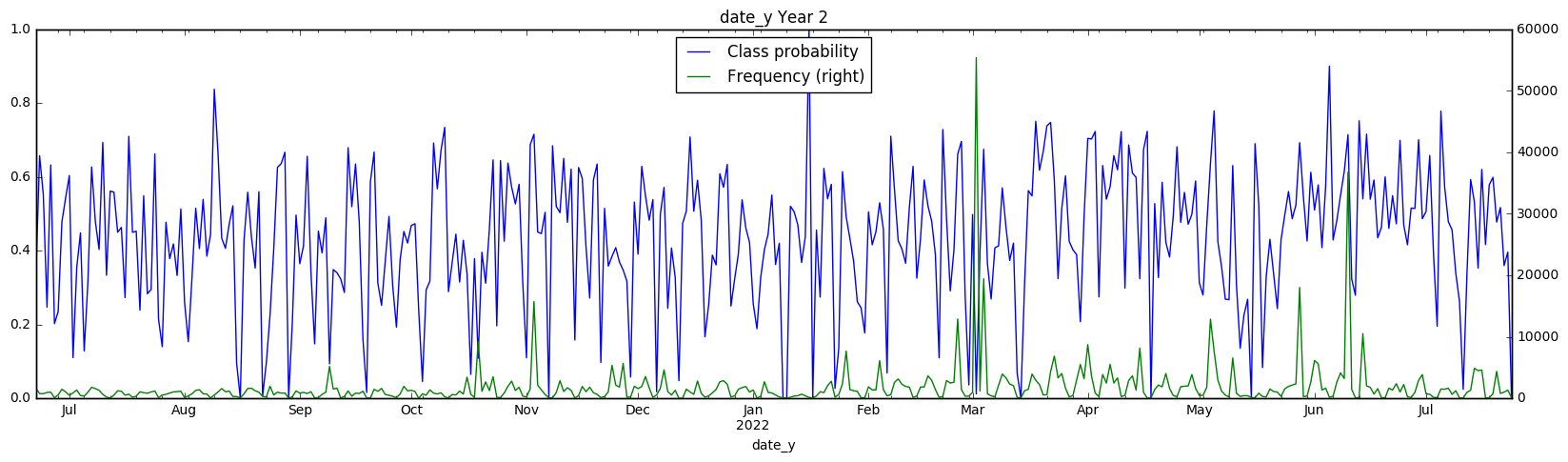
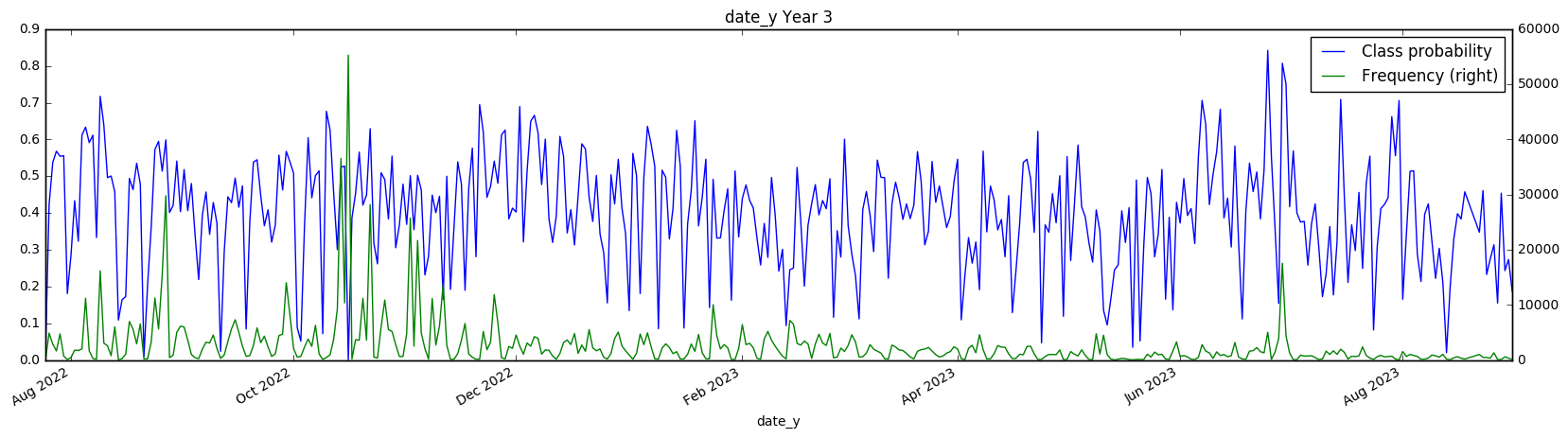
There also appears to be a weekly structure to the date_y variable, although it isn’t as cleanly visible. However, the class probabilities appear to swing much lower (reaching 0.2 on a weekly basis) We have to take these class probabilities with a grain of salt however, since we are hitting very low numbers of samples in each day with the date_y (in the hundreds). Test set However, all of this information is useless if the same pattern doesn’t emerge in the test set - let’s find out if this is the case! Since we don’t know the true class values, we can’t check if the same class probability appears in the test set, however we can check that the distribution of samples is the same.
date_x_freq = pd.DataFrame()
date_x_freq['Training set'] = df_train.groupby('date_x')['activity_id'].count()
date_x_freq['Testing set'] = df_test.groupby('date_x')['activity_id'].count()
date_x_freq.plot(secondary_y='Testing set', figsize=(20, 8),
                 title='Comparison of date_x distribution between training/testing set')
date_y_freq = pd.DataFrame()
date_y_freq['Training set'] = df_train.groupby('date_y')['activity_id'].count()
date_y_freq['Testing set'] = df_test.groupby('date_y')['activity_id'].count()
date_y_freq[:i].plot(secondary_y='Testing set', figsize=(20, 8),
                 title='Comparison of date_y distribution between training/testing set (first year)')
date_y_freq[2*i:].plot(secondary_y='Testing set', figsize=(20, 8),
                 title='Comparison of date_y distribution between training/testing set (last year)')
<matplotlib.axes._subplots.AxesSubplot at 0x7f6f59fbb940>
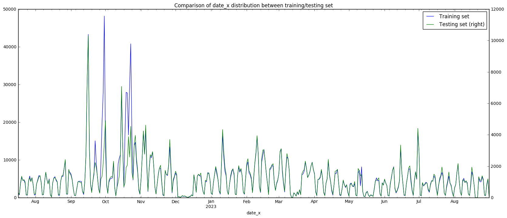
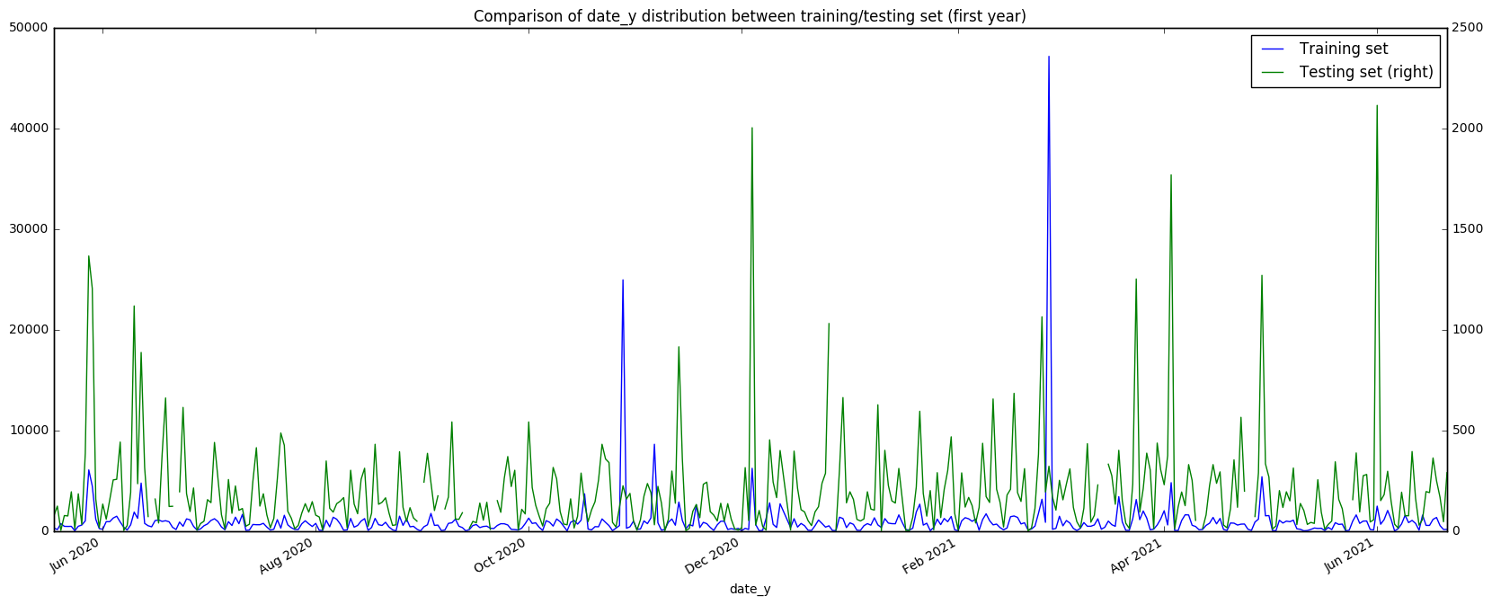
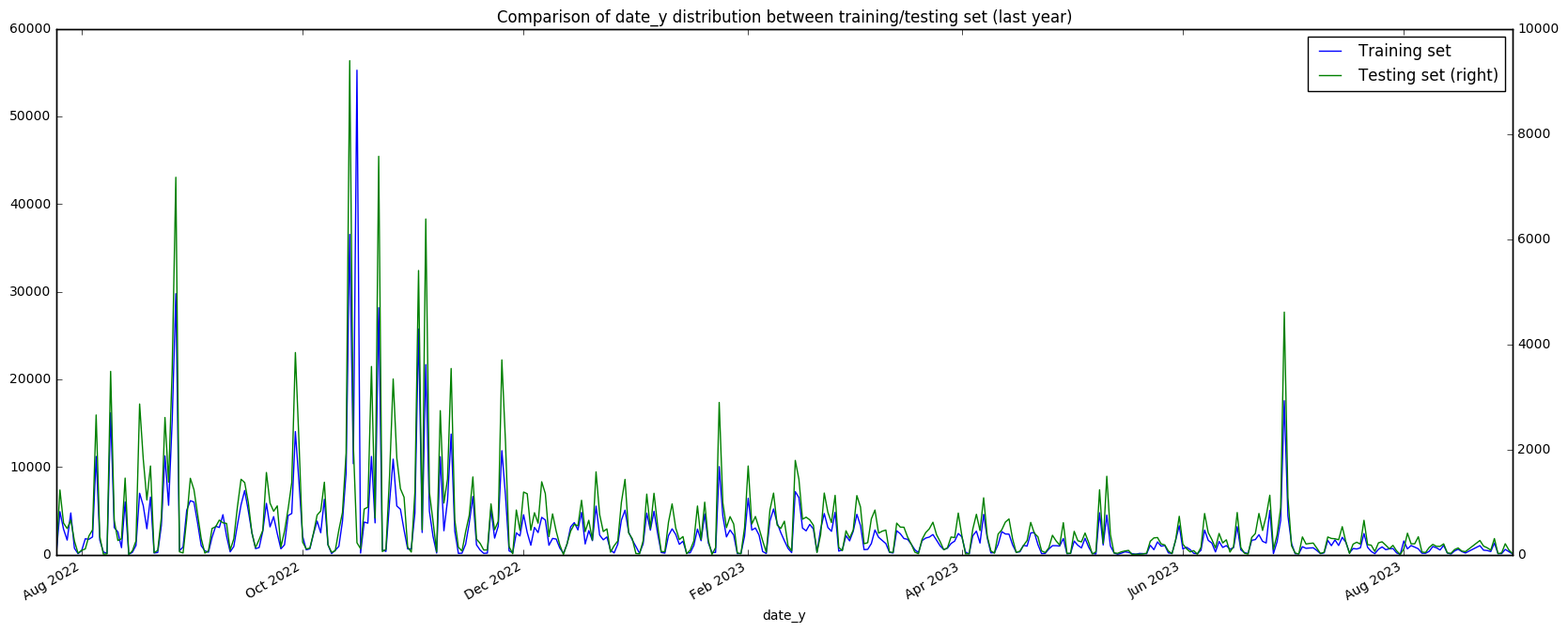
This gives us some interesting results. For date_x, we observe in the graph (and also in the high correlation value) that the training and testing sets have a very similar structure - this provides strong evidence that the training and testing sets are split based on people, and not based on time or some other unknown factor. Once again, we also observe the peaks (outliers?) in the September/October region. However, the date_y is less clear cut. There is a low correlation between the two sets, although there is definitely some relationship that we can see visually. There appears to be very many spikes in the test set in the first year (what could this mean?) That being said, in the last year of date_y the relationship between the two sets is much more apparent. Let’s try looking at the correlations over the years.
print('date_y correlation in year 1: ' + str(np.corrcoef(date_y_freq[:i].fillna(0).T)[0,1]))
print('date_y correlation in year 2: ' + str(np.corrcoef(date_y_freq[i:2*i].fillna(0).T)[0,1]))
print('date_y correlation in year 3: ' + str(np.corrcoef(date_y_freq[2*i:].fillna(0).T)[0,1]))
date_y correlation in year 1: 0.237056344324
date_y correlation in year 2: 0.682344221229
date_y correlation in year 3: 0.807207224857
Wow, that is definitely a huge improvement over time! Something about the structure of the first year of date_y doesn’t match up, so we should keep that in mind (If anyone has any theories I would love to hear them). Probability features To wrap up the first part of this EDA, I’m going to try turning the date class probabilities into features that we could use in our model, and then we can take a look at the AUCs that they give.
from sklearn.metrics import roc_auc_score
features = pd.DataFrame()
features['date_x_prob'] = df_train.groupby('date_x')['outcome'].transform('mean')
features['date_y_prob'] = df_train.groupby('date_y')['outcome'].transform('mean')
features['date_x_count'] = df_train.groupby('date_x')['outcome'].transform('count')
features['date_y_count'] = df_train.groupby('date_y')['outcome'].transform('count')
_=[print(f.ljust(12) + ' AUC: ' + str(round(roc_auc_score(df_train['outcome'], features[f]), 6))) for f in features.columns]
date_x_prob  AUC: 0.626182
date_y_prob  AUC: 0.720296
date_x_count AUC: 0.465697
date_y_count AUC: 0.475916
date_x_prob AUC: 0.626182 date_y_prob AUC: 0.720296 date_x_count AUC: 0.465697 date_y_count AUC: 0.475916 It looks like the date probability features have very high predictive power! I think we might be onto something here. Anyway, that’s all I’ve got for now. I’ll be back with more graphs and text soon, in the meantime if anyone has any theories or questions feel free to ask/discuss in the comments. Make sure to upvote if this was useful (and motivate me to make more!)
Here I would like to try XGBOOST to show how it is used.
import numpy as np
import pandas as pd
import xgboost as xgb
from sklearn.preprocessing import OneHotEncoder

def reduce_dimen(dataset,column,toreplace):
    for index,i in dataset[column].duplicated(keep=False).iteritems():
        if i==False:
            dataset.set_value(index,column,toreplace)
    return dataset

def act_data_treatment(dsname):
    dataset = dsname

    for col in list(dataset.columns):
        if col not in ['people_id', 'activity_id', 'date', 'char_38', 'outcome']:
            if dataset[col].dtype == 'object':
                dataset[col].fillna('type 0', inplace=True)
                dataset[col] = dataset[col].apply(lambda x: x.split(' ')[1]).astype(np.int32)
            elif dataset[col].dtype == 'bool':
                dataset[col] = dataset[col].astype(np.int8)

    dataset['year'] = dataset['date'].dt.year
    dataset['month'] = dataset['date'].dt.month
    dataset['day'] = dataset['date'].dt.day
    dataset['isweekend'] = (dataset['date'].dt.weekday >= 5).astype(int)
    dataset = dataset.drop('date', axis = 1)

    return dataset

act_train_data = pd.read_csv("../input/act_train.csv",dtype={'people_id': np.str, 'activity_id': np.str, 'outcome': np.int8}, parse_dates=['date'])
act_test_data  = pd.read_csv("../input/act_test.csv", dtype={'people_id': np.str, 'activity_id': np.str}, parse_dates=['date'])
people_data    = pd.read_csv("../input/people.csv", dtype={'people_id': np.str, 'activity_id': np.str, 'char_38': np.int32}, parse_dates=['date'])

act_train_data=act_train_data.drop('char_10',axis=1)
act_test_data=act_test_data.drop('char_10',axis=1)

print("Train data shape: " + format(act_train_data.shape))
print("Test data shape: " + format(act_test_data.shape))
print("People data shape: " + format(people_data.shape))

act_train_data  = act_data_treatment(act_train_data)
act_test_data   = act_data_treatment(act_test_data)
people_data = act_data_treatment(people_data)

train = act_train_data.merge(people_data, on='people_id', how='left', left_index=True)
test  = act_test_data.merge(people_data, on='people_id', how='left', left_index=True)

del act_train_data
del act_test_data
del people_data

train=train.sort_values(['people_id'], ascending=[1])
test=test.sort_values(['people_id'], ascending=[1])

train_columns = train.columns.values
test_columns = test.columns.values
features = list(set(train_columns) & set(test_columns))

train.fillna('NA', inplace=True)
test.fillna('NA', inplace=True)

y = train.outcome
train=train.drop('outcome',axis=1)

whole=pd.concat([train,test],ignore_index=True)
categorical=['group_1','activity_category','char_1_x','char_2_x','char_3_x','char_4_x','char_5_x','char_6_x','char_7_x','char_8_x','char_9_x','char_2_y','char_3_y','char_4_y','char_5_y','char_6_y','char_7_y','char_8_y','char_9_y']
for category in categorical:
    whole=reduce_dimen(whole,category,9999999)

X=whole[:len(train)]
X_test=whole[len(train):]

del train
del whole

X=X.sort_values(['people_id'], ascending=[1])

X = X[features].drop(['people_id', 'activity_id'], axis = 1)
X_test = X_test[features].drop(['people_id', 'activity_id'], axis = 1)

categorical=['group_1','activity_category','char_1_x','char_2_x','char_3_x','char_4_x','char_5_x','char_6_x','char_7_x','char_8_x','char_9_x','char_2_y','char_3_y','char_4_y','char_5_y','char_6_y','char_7_y','char_8_y','char_9_y']
not_categorical=[]
for category in X.columns:
    if category not in categorical:
        not_categorical.append(category)

enc = OneHotEncoder(handle_unknown='ignore')
enc=enc.fit(pd.concat([X[categorical],X_test[categorical]]))
X_cat_sparse=enc.transform(X[categorical])
X_test_cat_sparse=enc.transform(X_test[categorical])

from scipy.sparse import hstack
X_sparse=hstack((X[not_categorical], X_cat_sparse))
X_test_sparse=hstack((X_test[not_categorical], X_test_cat_sparse))

print("Training data: " + format(X_sparse.shape))
print("Test data: " + format(X_test_sparse.shape))
print("###########")
print("One Hot enconded Test Dataset Script")

dtrain = xgb.DMatrix(X_sparse,label=y)
dtest = xgb.DMatrix(X_test_sparse)

param = {'max_depth':10, 'eta':0.02, 'silent':1, 'objective':'binary:logistic' }
param['nthread'] = 4
param['eval_metric'] = 'auc'
param['subsample'] = 0.7
param['colsample_bytree']= 0.7
param['min_child_weight'] = 0
param['booster'] = "gblinear"

watchlist  = [(dtrain,'train')]
num_round = 300
early_stopping_rounds=10
bst = xgb.train(param, dtrain, num_round, watchlist,early_stopping_rounds=early_stopping_rounds)

ypred = bst.predict(dtest)
output = pd.DataFrame({ 'activity_id' : test['activity_id'], 'outcome': ypred })
output.head()
output.to_csv('without_leak.csv', index = False)
---------------------------------------------------------------------------

ImportError                               Traceback (most recent call last)

<ipython-input-12-3e4cc760390c> in <module>()
      1 import numpy as np
      2 import pandas as pd
----> 3 import xgboost as xgb
      4 from sklearn.preprocessing import OneHotEncoder
      5


ImportError: No module named 'xgboost'
The next part uses Keras
import pandas as pd
import numpy as np
from scipy import sparse as ssp
import pylab as plt
from sklearn.preprocessing import LabelEncoder,LabelBinarizer,MinMaxScaler,OneHotEncoder
from sklearn.feature_extraction.text import TfidfVectorizer,CountVectorizer
from sklearn.decomposition import TruncatedSVD,NMF,PCA,FactorAnalysis
from sklearn.feature_selection import SelectFromModel,SelectPercentile,f_classif
from sklearn.decomposition import TruncatedSVD
from sklearn.metrics import log_loss,roc_auc_score
from sklearn.pipeline import Pipeline,make_pipeline
from sklearn.cross_validation import StratifiedKFold,KFold
from keras.preprocessing import sequence
from keras.callbacks import ModelCheckpoint,Callback
from keras import backend as K
from keras.layers import Input, Embedding, LSTM, Dense,Flatten, Dropout, merge,Convolution1D,MaxPooling1D,Lambda,AveragePooling1D,Reshape
from keras.layers.normalization import BatchNormalization
from keras.optimizers import SGD
from keras.layers.advanced_activations import PReLU,LeakyReLU,ELU,SReLU
from keras.models import Model

seed = 1
np.random.seed(seed)
dim = 32
hidden=64


class AucCallback(Callback):  #inherits from Callback

    def __init__(self, validation_data=(), patience=25,is_regression=True,best_model_name='best_keras.mdl',feval='roc_auc_score',batch_size=1024*8):
        super(Callback, self).__init__()

        self.patience = patience
        self.X_val, self.y_val = validation_data  #tuple of validation X and y
        self.best = -np.inf
        self.wait = 0  #counter for patience
        self.best_model=None
        self.best_model_name = best_model_name
        self.is_regression = is_regression
        self.y_val = self.y_val#.astype(np.int)
        self.feval = feval
        self.batch_size = batch_size
    def on_epoch_end(self, epoch, logs={}):
        p = self.model.predict(self.X_val,batch_size=self.batch_size, verbose=0)#.ravel()
        if self.feval=='roc_auc_score':
            current = roc_auc_score(self.y_val,p)

        if current > self.best:
            self.best = current
            self.wait = 0
            self.model.save_weights(self.best_model_name,overwrite=True)


        else:
            if self.wait >= self.patience:
                self.model.stop_training = True
                print('Epoch %05d: early stopping' % (epoch))


            self.wait += 1 #incremental the number of times without improvement
        print('Epoch %d Auc: %f | Best Auc: %f \n' % (epoch,current,self.best))


def make_batches(size, batch_size):
    nb_batch = int(np.ceil(size/float(batch_size)))
    return [(i*batch_size, min(size, (i+1)*batch_size)) for i in range(0, nb_batch)]


def main():
    train = pd.read_csv('act_train.csv')
    test = pd.read_csv('act_test.csv')
    people = pd.read_csv('people.csv')
    columns = people.columns
    test['outcome'] = np.nan
    data = pd.concat([train,test])

    data = pd.merge(data,people,how='left',on='people_id').fillna('missing')
    train = data[:train.shape[0]]
    test = data[train.shape[0]:]


    columns = train.columns.tolist()
    columns.remove('activity_id')
    columns.remove('outcome')
    data = pd.concat([train,test])
    for c in columns:
        data[c] = LabelEncoder().fit_transform(data[c].values)

    train = data[:train.shape[0]]
    test = data[train.shape[0]:]

    data = pd.concat([train,test])
    columns = train.columns.tolist()
    columns.remove('activity_id')
    columns.remove('outcome')
    flatten_layers = []
    inputs = []
    count=0
    for c in columns:

        inputs_c = Input(shape=(1,), dtype='int32')

        num_c = len(np.unique(data[c].values))

        embed_c = Embedding(
                        num_c,
                        dim,
                        dropout=0.2,
                        input_length=1
                        )(inputs_c)
        flatten_c= Flatten()(embed_c)

        inputs.append(inputs_c)
        flatten_layers.append(flatten_c)
        count+=1

    flatten = merge(flatten_layers,mode='concat')
    reshaped_flatten = Reshape((count,dim))(flatten)

    conv_1 = Convolution1D(nb_filter=16,
                        filter_length=3,
                        border_mode='same',
                        activation='relu',
                        subsample_length=1)(reshaped_flatten)
    pool_1 = MaxPooling1D(pool_length=int(count/2))(conv_1)

    flatten = Flatten()(pool_1)


    fc1 = Dense(hidden,activation='relu')(flatten)
    dp1 = Dropout(0.5)(fc1)

    outputs = Dense(1,activation='sigmoid')(dp1)

    model = Model(input=inputs, output=outputs)
    model.compile(
                optimizer='adam',
                loss='binary_crossentropy',
              )

    del data

    X = train[columns].values
    X_t = test[columns].values
    y = train["outcome"].values
    people_id = train["people_id"].values
    activity_id = test['activity_id']
    del train
    del test

    skf = StratifiedKFold(y, n_folds=4, shuffle=True, random_state=seed)
    for ind_tr, ind_te in skf:
        X_train = X[ind_tr]
        X_test = X[ind_te]

        y_train = y[ind_tr]
        y_test = y[ind_te]
        break

    X_train = [X_train[:,i] for i in range(X.shape[1])]
    X_test = [X_test[:,i] for i in range(X.shape[1])]

    del X

    model_name = 'mlp_residual_%s_%s.hdf5'%(dim,hidden)
    model_checkpoint = ModelCheckpoint(model_name, monitor='val_loss', save_best_only=True)
    auc_callback = AucCallback(validation_data=(X_test,y_test), patience=5,is_regression=True,best_model_name='best_keras.mdl',feval='roc_auc_score')

    nb_epoch = 2

    batch_size = 1024*8
    load_model = False

    if load_model:
        print('Load Model')
        model.load_weights(model_name)
        # model.load_weights('best_keras.mdl')

    model.fit(
        X_train,
        y_train,
        batch_size=batch_size,
        nb_epoch=nb_epoch,
        verbose=1,
        shuffle=True,
        validation_data=[X_test,y_test],
        # callbacks = [
            # model_checkpoint,
            # auc_callback,
            # ],
        )

    # model.load_weights(model_name)
    # model.load_weights('best_keras.mdl')

    y_preds = model.predict(X_test,batch_size=1024*8)
    # print('auc',roc_auc_score(y_test,y_preds))

    # print('Make submission')
    X_t = [X_t[:,i] for i in range(X_t.shape[1])]
    outcome = model.predict(X_t,batch_size=1024*8)
    submission = pd.DataFrame()
    submission['activity_id'] = activity_id
    submission['outcome'] = outcome
    submission.to_csv('submission_residual_%s_%s.csv'%(dim,hidden),index=False)

main()
/home/dsno800/anaconda3/lib/python3.5/site-packages/tensorflow/python/ops/gradients.py:90: UserWarning: Converting sparse IndexedSlices to a dense Tensor of unknown shape. This may consume a large amount of memory.
  "Converting sparse IndexedSlices to a dense Tensor of unknown shape. "


Train on 1647967 samples, validate on 549324 samples
Epoch 1/2
1647967/1647967 [==============================] - 112s - loss: 0.3316 - val_loss: 0.0885
Epoch 2/2
1647967/1647967 [==============================] - 110s - loss: 0.1137 - val_loss: 0.0657
Here I just want to create an interesting matrix:
# Generate plots of:
# 411 columns: one per train/test day
# N rows: one per group (group_1 from people.csv)
# red pixels mean outcome for that group/day was 1, blue means 0

import pandas as pd
import numpy as np
from scipy.sparse import csr_matrix
from scipy.misc import imsave

def generatePixelPlot(df, name):
	print('creating', name)
	rows = []
	cols = []
	data = []
	groupIndex = -1
	prev = -1
	gb = df.groupby(['group_1', 'day_index'])
	for key, df in gb:
		if key[0]!=prev:
			prev = key[0]
			groupIndex += 1
		rows.append(groupIndex)
		cols.append(int(key[1]))
		# simple form of the leak: for a given group/day combination, take the maximum label
		# outcome will be -1, 0, or 1, shift that to 1, 2, 3
		data.append(df.outcome.max()+2)
	m = csr_matrix((data, (rows, cols)), dtype=np.int8)
	codes = m.toarray()
	full = np.zeros((m.shape[0], m.shape[1], 3), dtype=np.int8)
	full[...,0] = codes==3  # red channel is outcome 1
	full[...,2] = codes==2  # blue channel is outcome 0
	'''
	# alternative code to show test set group/day combination as white pixels
	full[...,0] = np.logical_or(codes==1, codes==3)
	full[...,1] = (codes==1)
	full[...,2] = np.logical_or(codes==1, codes==2)
	'''
	imsave(name, full)


people = pd.read_csv("people.csv", usecols=['people_id','group_1'])
people['group_1'] = people['group_1'].apply(lambda s: int(s[s.find(' ')+1:])).astype(int)

train = pd.read_csv("act_train.csv", usecols=['people_id','date','outcome'], parse_dates=['date'])
test = pd.read_csv("act_test.csv", usecols=['people_id','date'], parse_dates=['date'])
test['outcome'] = -1
all = train.append(test)

# make index of days 0..410
epoch = all.date.min()
all['day_index'] = (all['date'] - epoch) / np.timedelta64(1, 'D')

# add group_1 to main DataFrame & sort by it
all = pd.merge(all, people, on='people_id', how='left')
all = all.sort_values('group_1')

# create pixel plots for all groups, in 411x2000 chunks (2000 groups at a time)
groups = all.group_1.unique()
offset = 0
count = 2000
while offset < len(groups):
	sub = groups[offset:offset + count]
	generatePixelPlot(all.ix[all.group_1.isin(sub)], 'groups_%05d_to_%05d.png'%(sub.min(), sub.max()))
	offset += count

# special case: for all (4253) groups that switch outcome over time
# are there any patterns in the timing of changes?
gb = all.groupby('group_1')
switchers = gb.outcome.apply(lambda x: 0 in x.values and 1 in x.values)
groups = set(switchers.ix[switchers].index)
print('#switchers:', len(groups))
generatePixelPlot(all.ix[all.group_1.isin(groups)], 'switcher_groups.png')
creating groups_00001_to_02420.png
creating groups_02421_to_05178.png
creating groups_05179_to_07952.png
creating groups_07953_to_10946.png
creating groups_10948_to_14111.png
creating groups_14113_to_17306.png
creating groups_17307_to_19897.png
creating groups_19898_to_22602.png
creating groups_22603_to_25410.png
creating groups_25411_to_28348.png
creating groups_28350_to_31348.png
creating groups_31350_to_34586.png
creating groups_34588_to_37742.png
creating groups_37743_to_40955.png
creating groups_40956_to_44220.png
creating groups_44222_to_47628.png
creating groups_47629_to_51077.png
creating groups_51080_to_51462.png
#switchers: 4253
creating switcher_groups.png
What follows is an awesome date trick that can be achieved
# --- original script author's comments.
## --- Alex Ilchenko's comments.

import pandas as pd
import numpy as np
import datetime
from itertools import product
from scipy import interpolate ## For other interpolation functions.

def interpolateFun0(x):
    """Original script author's function rewritten in Python.
    The author interpolates between two known values by averaging them. We
    can think of this as 0th order interpolation. """

    ## TODO: This function could use some optimization. The R version is much faster...
    x = x.reset_index(drop=True)
    g = x['outcome'] ## g should be a list or a pandas Series.
    if g.shape[0] < 3: ## If we have at most two rows.
        x['filled'] = g ## Will be replaced by a mean.
        return x
    missing_index = g.isnull()
    borders = np.append([g.index[0]], g[~missing_index].index, axis=0)
    borders = np.append(borders, [g.index[-1]+1], axis=0)
    forward_border = borders[1:]
    backward_border = borders[:-1]
    forward_border_g = g[forward_border]
    backward_border_g = g[backward_border]
    ## Interpolate borders.
    ## TODO: Why does the script author use the value 0.1?
    border_fill = 0.1
    forward_border_g[forward_border_g.index[-1]] = abs(forward_border_g[forward_border_g.index[-2]]-border_fill)
    backward_border_g[backward_border_g.index[0]] = abs(forward_border_g[forward_border_g.index[0]]-border_fill)
    times = forward_border-backward_border
    forward_x_fill = np.repeat(forward_border_g, times).reset_index(drop=True)
    backward_x_fill = np.repeat(backward_border_g, times).reset_index(drop=True)
    vec = (forward_x_fill+backward_x_fill)/2
    g[missing_index] = vec[missing_index] ## Impute missing values only.
    x['filled'] = g
    return x

def interpolateFun1(x):
    """First-order interpolation between known values. """
    g = x['outcome']
    missing_index = g.isnull()
    border_fill = 0.1 ## TODO: Shouldn't this be some kind of a mean value for the group?
    #border_fill = g.mean() ## Uncomment to try a different border fill.
    if g.index[0] in missing_index:
        g[g.index[0]] = border_fill
    if g.index[-1] in missing_index:
        g[g.index[-1]] = border_fill
    known_index = ~g.isnull()
    try:
        f = interpolate.interp1d(g[known_index].index, g[known_index], kind='linear')
        x['filled'] = [f(x) for x in g.index]
        x['filled'] = np.interp(g.index, g[known_index].index, g[known_index])
    except ValueError:
        x['filled'] = x['outcome']
    return x

if __name__ == '__main__':
    # Load and transform people data. ----------------------------------------------
    ppl = pd.read_csv('people.csv')

    # Convert booleans to integers.
    p_logi = ppl.select_dtypes(include=['bool']).columns
    ppl[p_logi] = ppl[p_logi].astype('int')
    del p_logi

    # Transform date.
    ppl['date'] = pd.to_datetime(ppl['date'])

    # Load activities.--------------------------------------------------------------
    # Read and combine.
    activs = pd.read_csv('act_train.csv')
    TestActivs = pd.read_csv('act_test.csv')
    TestActivs['outcome'] = np.nan ## Add the missing column to the test set.
    activs = pd.concat([activs, TestActivs], axis=0) ## Append train and test sets.
    del TestActivs

    # Extract only required variables.
    activs = activs[['people_id', 'outcome', 'activity_id', 'date']] ## Let's look at these columns only.

    # Merge people data into activities.
    ## This keeps all the rows from activities.
    ## TODO: We are not using rows from ppl who have no activities...
    d1 = pd.merge(activs, ppl, on='people_id', how='right')

    ## These are the indices of the rows from the test set.
    testset = ppl[ppl['people_id'].isin(d1[d1['outcome'].isnull()]['people_id'])].index

    d1['activdate'] = pd.to_datetime(d1['date_x'])

    del activs

    # Prepare grid for prediction. -------------------------------------------------

    # Create all group_1/day grid.
    minactivdate = min(d1['activdate'])
    maxactivdate = max(d1['activdate'])

    ## Make a list of all days from min to max.
    alldays = [maxactivdate - datetime.timedelta(days=x) for x in range(0, (maxactivdate - minactivdate).days+1)][::-1]

    ## Take the values of group_1 from the rows of d1 which do not belong to the test set.
    grid_left = set(d1[~d1['people_id'].isin(ppl.iloc[testset]['people_id'])]['group_1'])
    ## Take cartesian product between the above variable and the list of all days.
    ## I think in the original script author thinks of the values in group_1 as companies.
    allCompaniesAndDays = pd.DataFrame.from_records(product(grid_left, alldays))

    # Nicer names.
    allCompaniesAndDays.columns = ['group_1', 'date_p']

    # Sort it.
    allCompaniesAndDays.sort_values(['group_1', 'date_p'], inplace=True)

    ## This is what allCompaniesAndDays looks like so far.
    """
    >>> allCompaniesAndDays.sample(n=10)
                  group_1     date_p
    10318543  group 14386 2023-08-09
    3470112    group 8767 2022-08-25
    5542924   group 30061 2023-01-11
    2328370   group 39750 2022-09-10
    7764760    group 1175 2022-12-12
    4788523    group 3788 2023-07-25
    5545711   group 12085 2022-10-13
    859359    group 28900 2023-07-21
    11188454  group 21110 2023-02-14
    9277889   group 26980 2023-08-07
    """

    # What are values on days where we have data?
    ## For a combination of group_1 and activdate, calculate the mean of the outcome variable.
    meanbycomdate = d1[~d1['people_id'].isin(ppl.iloc[testset]['people_id'])].groupby(['group_1', 'activdate'])['outcome'].agg('mean')
    ## Convert the calculation into a proper DataFrame.
    meanbycomdate = meanbycomdate.to_frame().reset_index()

    # Add them to full data grid.
    allCompaniesAndDays = pd.merge(allCompaniesAndDays, meanbycomdate, left_on=['group_1', 'date_p'], right_on=['group_1', 'activdate'], how='left')
    allCompaniesAndDays.drop('activdate', axis=1, inplace=True)
    allCompaniesAndDays.sort_values(['group_1', 'date_p'], inplace=True)

    ## This is what allCompaniesAndDays looks like so far.
    """
    >>> allCompaniesAndDays.sample(n=10)
                  group_1     date_p  outcome
    9536947   group 45684 2022-10-28      NaN
    11989016   group 8966 2022-12-10      NaN
    11113251   group 6012 2023-02-24      NaN
    9945551    group 4751 2023-01-06      1.0
    2273368   group 18350 2022-11-21      NaN
    12276013   group 9956 2023-04-08      NaN
    371765    group 11362 2023-02-23      NaN
    10065054  group 48049 2022-09-30      NaN
    5525397   group 29428 2023-06-06      NaN
    4911409   group 27233 2023-07-22      NaN
    """

    ## Add a column 'filled' which gives the imputed values for missing values in column 'outcome'.
    # groups = [df for _, df in list(allCompaniesAndDays.groupby('group_1'))]
    # dfs = [interpolateFun1(group) for group in groups]
    # allCompaniesAndDays = pd.concat(dfs)
    # allCompaniesAndDays.reset_index(drop=True, inplace=True)

    allCompaniesAndDays = allCompaniesAndDays.groupby('group_1').apply(interpolateFun0)

    d1 = pd.merge(d1, allCompaniesAndDays,
                  left_on=['group_1', 'activdate'], right_on=['group_1', 'date_p'], how='left')

    testsetdt = d1[d1['people_id'].isin(ppl.iloc[testset]['people_id'])][['activity_id', 'filled']]
    ## There are no NAs.
    testsetdt.columns = [testsetdt.columns[0], 'outcome']
    testsetdt['outcome'] = testsetdt['outcome'].fillna(testsetdt['outcome'].mean())
    testsetdt.to_csv('Submission.csv', index=False)