Credit Card Fraud Model
Estimated reading time: 53 minutesCredit Card Fraud Model
import pandas as pd
import matplotlib.pyplot as plt
import numpy as np
df = pd.read_csv('creditcard.csv')
df.head()
| Time | V1 | V2 | V3 | V4 | V5 | V6 | V7 | V8 | V9 | V10 | V11 | V12 | V13 | V14 | V15 | V16 | V17 | V18 | V19 | V20 | V21 | V22 | V23 | V24 | V25 | V26 | V27 | V28 | Amount | Class | |
|---|---|---|---|---|---|---|---|---|---|---|---|---|---|---|---|---|---|---|---|---|---|---|---|---|---|---|---|---|---|---|---|
| 0 | 0.0 | -1.359807 | -0.072781 | 2.536347 | 1.378155 | -0.338321 | 0.462388 | 0.239599 | 0.098698 | 0.363787 | 0.090794 | -0.551600 | -0.617801 | -0.991390 | -0.311169 | 1.468177 | -0.470401 | 0.207971 | 0.025791 | 0.403993 | 0.251412 | -0.018307 | 0.277838 | -0.110474 | 0.066928 | 0.128539 | -0.189115 | 0.133558 | -0.021053 | 149.62 | 0 |
| 1 | 0.0 | 1.191857 | 0.266151 | 0.166480 | 0.448154 | 0.060018 | -0.082361 | -0.078803 | 0.085102 | -0.255425 | -0.166974 | 1.612727 | 1.065235 | 0.489095 | -0.143772 | 0.635558 | 0.463917 | -0.114805 | -0.183361 | -0.145783 | -0.069083 | -0.225775 | -0.638672 | 0.101288 | -0.339846 | 0.167170 | 0.125895 | -0.008983 | 0.014724 | 2.69 | 0 |
| 2 | 1.0 | -1.358354 | -1.340163 | 1.773209 | 0.379780 | -0.503198 | 1.800499 | 0.791461 | 0.247676 | -1.514654 | 0.207643 | 0.624501 | 0.066084 | 0.717293 | -0.165946 | 2.345865 | -2.890083 | 1.109969 | -0.121359 | -2.261857 | 0.524980 | 0.247998 | 0.771679 | 0.909412 | -0.689281 | -0.327642 | -0.139097 | -0.055353 | -0.059752 | 378.66 | 0 |
| 3 | 1.0 | -0.966272 | -0.185226 | 1.792993 | -0.863291 | -0.010309 | 1.247203 | 0.237609 | 0.377436 | -1.387024 | -0.054952 | -0.226487 | 0.178228 | 0.507757 | -0.287924 | -0.631418 | -1.059647 | -0.684093 | 1.965775 | -1.232622 | -0.208038 | -0.108300 | 0.005274 | -0.190321 | -1.175575 | 0.647376 | -0.221929 | 0.062723 | 0.061458 | 123.50 | 0 |
| 4 | 2.0 | -1.158233 | 0.877737 | 1.548718 | 0.403034 | -0.407193 | 0.095921 | 0.592941 | -0.270533 | 0.817739 | 0.753074 | -0.822843 | 0.538196 | 1.345852 | -1.119670 | 0.175121 | -0.451449 | -0.237033 | -0.038195 | 0.803487 | 0.408542 | -0.009431 | 0.798278 | -0.137458 | 0.141267 | -0.206010 | 0.502292 | 0.219422 | 0.215153 | 69.99 | 0 |
The variables in this dataset is not very informative, even though we know the variables relates to credit card transactions the the data has been annonimised.
%matplotlib inline
# This means that it actually shows the plot
count_classes = pd.value_counts(df['Class'], sort = True).sort_index()
count_classes.plot(kind = 'bar', color="purple")
plt.title("Fraud class histogram")
plt.xlabel("Class")
plt.ylabel("Frequency")
<matplotlib.text.Text at 0x7fbdd2b3c278>
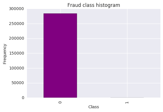
The data is clearly unbalanced and the amount of legitimate transactions far outdo the fraudulent transactions. This type of data should be analysed with absolute care due to the high benchmark accuracy achieved from merely selecting the most frequently occured target class.
A few of the possible strategies is to:
- Use the confusion matrix to calculate Precision and Recall.
- F1score (The weighted average of precision recall)
- Usae Kappa - This is the classification accuracy normalised by the imabalnce of the classes in the data.
-
ROC curves to calculate the sensitivity/specificity ratio.
- There is also the possibility of resampling the data so that it has an approximate 50-50 ratio.
- The easiest way to do this is by over-sampling which merely means to include additional copies of the under-represented class (preferred strategy when you have little data)
- Another possible method linked with the above concept is to undersample, which deletes instances from the over-represented class (preferred strategy when you have lots of data)
Hybrid approach:
Apart from the above mentioned methods to resample skewed data you can also use the SMOTE (Synthetic Minority Over-Sampling Technique), which is a combination of the over and under sampling technique. The oversampling is done by constructing new minority class data via an algorithm.
df.describe()
| Time | V1 | V2 | V3 | V4 | V5 | V6 | V7 | V8 | V9 | V10 | V11 | V12 | V13 | V14 | V15 | V16 | V17 | V18 | V19 | V20 | V21 | V22 | V23 | V24 | V25 | V26 | V27 | V28 | Amount | Class | |
|---|---|---|---|---|---|---|---|---|---|---|---|---|---|---|---|---|---|---|---|---|---|---|---|---|---|---|---|---|---|---|---|
| count | 284807.000000 | 2.848070e+05 | 2.848070e+05 | 2.848070e+05 | 2.848070e+05 | 2.848070e+05 | 2.848070e+05 | 2.848070e+05 | 2.848070e+05 | 2.848070e+05 | 2.848070e+05 | 2.848070e+05 | 2.848070e+05 | 2.848070e+05 | 2.848070e+05 | 2.848070e+05 | 2.848070e+05 | 2.848070e+05 | 2.848070e+05 | 2.848070e+05 | 2.848070e+05 | 2.848070e+05 | 2.848070e+05 | 2.848070e+05 | 2.848070e+05 | 2.848070e+05 | 2.848070e+05 | 2.848070e+05 | 2.848070e+05 | 284807.000000 | 284807.000000 |
| mean | 94813.859575 | 3.919560e-15 | 5.688174e-16 | -8.769071e-15 | 2.782312e-15 | -1.552563e-15 | 2.010663e-15 | -1.694249e-15 | -1.927028e-16 | -3.137024e-15 | 1.768627e-15 | 9.170318e-16 | -1.810658e-15 | 1.693438e-15 | 1.479045e-15 | 3.482336e-15 | 1.392007e-15 | -7.528491e-16 | 4.328772e-16 | 9.049732e-16 | 5.085503e-16 | 1.537294e-16 | 7.959909e-16 | 5.367590e-16 | 4.458112e-15 | 1.453003e-15 | 1.699104e-15 | -3.660161e-16 | -1.206049e-16 | 88.349619 | 0.001727 |
| std | 47488.145955 | 1.958696e+00 | 1.651309e+00 | 1.516255e+00 | 1.415869e+00 | 1.380247e+00 | 1.332271e+00 | 1.237094e+00 | 1.194353e+00 | 1.098632e+00 | 1.088850e+00 | 1.020713e+00 | 9.992014e-01 | 9.952742e-01 | 9.585956e-01 | 9.153160e-01 | 8.762529e-01 | 8.493371e-01 | 8.381762e-01 | 8.140405e-01 | 7.709250e-01 | 7.345240e-01 | 7.257016e-01 | 6.244603e-01 | 6.056471e-01 | 5.212781e-01 | 4.822270e-01 | 4.036325e-01 | 3.300833e-01 | 250.120109 | 0.041527 |
| min | 0.000000 | -5.640751e+01 | -7.271573e+01 | -4.832559e+01 | -5.683171e+00 | -1.137433e+02 | -2.616051e+01 | -4.355724e+01 | -7.321672e+01 | -1.343407e+01 | -2.458826e+01 | -4.797473e+00 | -1.868371e+01 | -5.791881e+00 | -1.921433e+01 | -4.498945e+00 | -1.412985e+01 | -2.516280e+01 | -9.498746e+00 | -7.213527e+00 | -5.449772e+01 | -3.483038e+01 | -1.093314e+01 | -4.480774e+01 | -2.836627e+00 | -1.029540e+01 | -2.604551e+00 | -2.256568e+01 | -1.543008e+01 | 0.000000 | 0.000000 |
| 25% | 54201.500000 | -9.203734e-01 | -5.985499e-01 | -8.903648e-01 | -8.486401e-01 | -6.915971e-01 | -7.682956e-01 | -5.540759e-01 | -2.086297e-01 | -6.430976e-01 | -5.354257e-01 | -7.624942e-01 | -4.055715e-01 | -6.485393e-01 | -4.255740e-01 | -5.828843e-01 | -4.680368e-01 | -4.837483e-01 | -4.988498e-01 | -4.562989e-01 | -2.117214e-01 | -2.283949e-01 | -5.423504e-01 | -1.618463e-01 | -3.545861e-01 | -3.171451e-01 | -3.269839e-01 | -7.083953e-02 | -5.295979e-02 | 5.600000 | 0.000000 |
| 50% | 84692.000000 | 1.810880e-02 | 6.548556e-02 | 1.798463e-01 | -1.984653e-02 | -5.433583e-02 | -2.741871e-01 | 4.010308e-02 | 2.235804e-02 | -5.142873e-02 | -9.291738e-02 | -3.275735e-02 | 1.400326e-01 | -1.356806e-02 | 5.060132e-02 | 4.807155e-02 | 6.641332e-02 | -6.567575e-02 | -3.636312e-03 | 3.734823e-03 | -6.248109e-02 | -2.945017e-02 | 6.781943e-03 | -1.119293e-02 | 4.097606e-02 | 1.659350e-02 | -5.213911e-02 | 1.342146e-03 | 1.124383e-02 | 22.000000 | 0.000000 |
| 75% | 139320.500000 | 1.315642e+00 | 8.037239e-01 | 1.027196e+00 | 7.433413e-01 | 6.119264e-01 | 3.985649e-01 | 5.704361e-01 | 3.273459e-01 | 5.971390e-01 | 4.539234e-01 | 7.395934e-01 | 6.182380e-01 | 6.625050e-01 | 4.931498e-01 | 6.488208e-01 | 5.232963e-01 | 3.996750e-01 | 5.008067e-01 | 4.589494e-01 | 1.330408e-01 | 1.863772e-01 | 5.285536e-01 | 1.476421e-01 | 4.395266e-01 | 3.507156e-01 | 2.409522e-01 | 9.104512e-02 | 7.827995e-02 | 77.165000 | 0.000000 |
| max | 172792.000000 | 2.454930e+00 | 2.205773e+01 | 9.382558e+00 | 1.687534e+01 | 3.480167e+01 | 7.330163e+01 | 1.205895e+02 | 2.000721e+01 | 1.559499e+01 | 2.374514e+01 | 1.201891e+01 | 7.848392e+00 | 7.126883e+00 | 1.052677e+01 | 8.877742e+00 | 1.731511e+01 | 9.253526e+00 | 5.041069e+00 | 5.591971e+00 | 3.942090e+01 | 2.720284e+01 | 1.050309e+01 | 2.252841e+01 | 4.584549e+00 | 7.519589e+00 | 3.517346e+00 | 3.161220e+01 | 3.384781e+01 | 25691.160000 | 1.000000 |
I am goin to standardise all the variables, they do not look good, especially the amount column.
from sklearn.preprocessing import StandardScaler
df = pd.read_csv('creditcard.csv')
time = df["Time"]
classes = df["Class"]
df.pop("Time")
df.pop("Class")
listed = list(df)
data = StandardScaler().fit_transform(df)

#data = data.drop(['Time','Amount'],axis=1)
#data.head()
df = pd.DataFrame(data)
df.columns = listed
df["Time"] = time
df["Class"] = classes
df.describe()
| V1 | V2 | V3 | V4 | V5 | V6 | V7 | V8 | V9 | V10 | V11 | V12 | V13 | V14 | V15 | V16 | V17 | V18 | V19 | V20 | V21 | V22 | V23 | V24 | V25 | V26 | V27 | V28 | Amount | Time | Class | |
|---|---|---|---|---|---|---|---|---|---|---|---|---|---|---|---|---|---|---|---|---|---|---|---|---|---|---|---|---|---|---|---|
| count | 2.848070e+05 | 2.848070e+05 | 2.848070e+05 | 2.848070e+05 | 2.848070e+05 | 2.848070e+05 | 2.848070e+05 | 2.848070e+05 | 2.848070e+05 | 2.848070e+05 | 2.848070e+05 | 2.848070e+05 | 2.848070e+05 | 2.848070e+05 | 2.848070e+05 | 2.848070e+05 | 2.848070e+05 | 2.848070e+05 | 2.848070e+05 | 2.848070e+05 | 2.848070e+05 | 2.848070e+05 | 2.848070e+05 | 2.848070e+05 | 2.848070e+05 | 2.848070e+05 | 2.848070e+05 | 2.848070e+05 | 2.848070e+05 | 284807.000000 | 284807.000000 |
| mean | -8.157366e-16 | 3.154853e-17 | -4.409878e-15 | -6.734811e-16 | -2.874435e-16 | 4.168992e-16 | -8.767997e-16 | -2.423604e-16 | 3.078727e-16 | 2.026926e-17 | 1.622758e-15 | 2.052953e-15 | -8.310622e-17 | -8.845502e-16 | -1.789241e-15 | -1.542079e-16 | 8.046919e-16 | -2.547965e-16 | -4.550555e-16 | 2.754870e-16 | 1.685077e-17 | 1.478472e-15 | -6.797197e-16 | 1.234659e-16 | -7.659279e-16 | 3.247603e-16 | -2.953495e-18 | 5.401572e-17 | 3.202236e-16 | 94813.859575 | 0.001727 |
| std | 1.000002e+00 | 1.000002e+00 | 1.000002e+00 | 1.000002e+00 | 1.000002e+00 | 1.000002e+00 | 1.000002e+00 | 1.000002e+00 | 1.000002e+00 | 1.000002e+00 | 1.000002e+00 | 1.000002e+00 | 1.000002e+00 | 1.000002e+00 | 1.000002e+00 | 1.000002e+00 | 1.000002e+00 | 1.000002e+00 | 1.000002e+00 | 1.000002e+00 | 1.000002e+00 | 1.000002e+00 | 1.000002e+00 | 1.000002e+00 | 1.000002e+00 | 1.000002e+00 | 1.000002e+00 | 1.000002e+00 | 1.000002e+00 | 47488.145955 | 0.041527 |
| min | -2.879855e+01 | -4.403529e+01 | -3.187173e+01 | -4.013919e+00 | -8.240810e+01 | -1.963606e+01 | -3.520940e+01 | -6.130252e+01 | -1.222802e+01 | -2.258191e+01 | -4.700128e+00 | -1.869868e+01 | -5.819392e+00 | -2.004428e+01 | -4.915191e+00 | -1.612534e+01 | -2.962645e+01 | -1.133266e+01 | -8.861402e+00 | -7.069146e+01 | -4.741907e+01 | -1.506565e+01 | -7.175446e+01 | -4.683638e+00 | -1.975033e+01 | -5.401098e+00 | -5.590660e+01 | -4.674612e+01 | -3.532294e-01 | 0.000000 | 0.000000 |
| 25% | -4.698918e-01 | -3.624707e-01 | -5.872142e-01 | -5.993788e-01 | -5.010686e-01 | -5.766822e-01 | -4.478860e-01 | -1.746805e-01 | -5.853631e-01 | -4.917360e-01 | -7.470224e-01 | -4.058964e-01 | -6.516198e-01 | -4.439565e-01 | -6.368132e-01 | -5.341353e-01 | -5.695609e-01 | -5.951621e-01 | -5.605369e-01 | -2.746334e-01 | -3.109433e-01 | -7.473476e-01 | -2.591784e-01 | -5.854676e-01 | -6.084001e-01 | -6.780717e-01 | -1.755053e-01 | -1.604440e-01 | -3.308401e-01 | 54201.500000 | 0.000000 |
| 50% | 9.245351e-03 | 3.965683e-02 | 1.186124e-01 | -1.401724e-02 | -3.936682e-02 | -2.058046e-01 | 3.241723e-02 | 1.871982e-02 | -4.681169e-02 | -8.533551e-02 | -3.209268e-02 | 1.401448e-01 | -1.363250e-02 | 5.278702e-02 | 5.251917e-02 | 7.579255e-02 | -7.732604e-02 | -4.338370e-03 | 4.588014e-03 | -8.104705e-02 | -4.009429e-02 | 9.345377e-03 | -1.792420e-02 | 6.765678e-02 | 3.183240e-02 | -1.081217e-01 | 3.325174e-03 | 3.406368e-02 | -2.652715e-01 | 84692.000000 | 0.000000 |
| 75% | 6.716939e-01 | 4.867202e-01 | 6.774569e-01 | 5.250082e-01 | 4.433465e-01 | 2.991625e-01 | 4.611107e-01 | 2.740785e-01 | 5.435305e-01 | 4.168842e-01 | 7.245863e-01 | 6.187332e-01 | 6.656518e-01 | 5.144513e-01 | 7.088502e-01 | 5.971989e-01 | 4.705737e-01 | 5.974968e-01 | 5.637928e-01 | 1.725733e-01 | 2.537392e-01 | 7.283360e-01 | 2.364319e-01 | 7.257153e-01 | 6.728006e-01 | 4.996663e-01 | 2.255648e-01 | 2.371526e-01 | -4.471707e-02 | 139320.500000 | 0.000000 |
| max | 1.253351e+00 | 1.335775e+01 | 6.187993e+00 | 1.191874e+01 | 2.521413e+01 | 5.502015e+01 | 9.747824e+01 | 1.675153e+01 | 1.419494e+01 | 2.180758e+01 | 1.177504e+01 | 7.854679e+00 | 7.160735e+00 | 1.098147e+01 | 9.699117e+00 | 1.976044e+01 | 1.089502e+01 | 6.014342e+00 | 6.869414e+00 | 5.113464e+01 | 3.703471e+01 | 1.447304e+01 | 3.607668e+01 | 7.569684e+00 | 1.442532e+01 | 7.293975e+00 | 7.831940e+01 | 1.025434e+02 | 1.023622e+02 | 172792.000000 | 1.000000 |
The data looks much better after the standard scaler has been tun through.
# Okay now to fix the skewness:

data = df

X = data.ix[:, data.columns != 'Class']
y = data.ix[:, data.columns == 'Class']
# Number of data points in the minority class
number_records_fraud = len(data[data.Class == 1])
fraud_indices = np.array(data[data.Class == 1].index)

# Picking the indices of the normal classes
normal_indices = data[data.Class == 0].index

# Out of the indices we picked, randomly select "x" number (number_records_fraud)
random_normal_indices = np.random.choice(normal_indices, number_records_fraud, replace = False)
random_normal_indices = np.array(random_normal_indices)

# Appending the 2 indices
under_sample_indices = np.concatenate([fraud_indices,random_normal_indices])

# Under sample dataset
under_sample_data = data.iloc[under_sample_indices,:]

X_undersample = under_sample_data.ix[:, under_sample_data.columns != 'Class']
y_undersample = under_sample_data.ix[:, under_sample_data.columns == 'Class']

# Showing ratio
print("Percentage of normal transactions: ", len(under_sample_data[under_sample_data.Class == 0])/len(under_sample_data))
print("Percentage of fraud transactions: ", len(under_sample_data[under_sample_data.Class == 1])/len(under_sample_data))
print("Total number of transactions in resampled data: ", len(under_sample_data))
Percentage of normal transactions:  0.5
Percentage of fraud transactions:  0.5
Total number of transactions in resampled data:  984
from sklearn.cross_validation import train_test_split

# Whole dataset
X_train, X_test, y_train, y_test = train_test_split(X,y,test_size = 0.3, random_state = 0)

print("Number transactions train dataset: ", len(X_train))
print("Number transactions test dataset: ", len(X_test))
print("Total number of transactions: ", len(X_train)+len(X_test))

# Undersampled dataset
X_train_undersample, X_test_undersample, y_train_undersample, y_test_undersample = train_test_split(X_undersample
                                                                                                   ,y_undersample
                                                                                                   ,test_size = 0.3
                                                                                                   ,random_state = 0)
print("")
print("Number transactions train dataset: ", len(X_train_undersample))
print("Number transactions test dataset: ", len(X_test_undersample))
print("Total number of transactions: ", len(X_train_undersample)+len(X_test_undersample))
Number transactions train dataset:  199364
Number transactions test dataset:  85443
Total number of transactions:  284807

Number transactions train dataset:  688
Number transactions test dataset:  296
Total number of transactions:  984
We are very interested in the recall score, because that is the metric that will help us try to capture the most fraudulent transactions. If you think how Accuracy, Precision and Recall work for a confusion matrix, recall would be the most interesting:
Accuracy = (TP+TN)/total Precision = TP/(TP+FP) Recall = TP/(TP+FN)
As we know, due to the imbalacing of the data, many observations could be predicted as False Negatives, being, that we predict a normal transaction, but it is in fact a fraudulent one. Recall captures this.
Obviously, trying to increase recall, tends to come with a decrease of precision. However, in our case, if we predict that a transaction is fraudulent and turns out not to be, is not a massive problem compared to the opposite.
We could even apply a cost function when having FN and FP with different weights for each type of error, but let’s leave that aside for now.
from sklearn.linear_model import LogisticRegression
from sklearn.cross_validation import KFold, cross_val_score
from sklearn.metrics import confusion_matrix,precision_recall_curve,auc,roc_auc_score,roc_curve,recall_score,classification_report
def printing_Kfold_scores(x_train_data,y_train_data):
    fold = KFold(len(y_train_data),5,shuffle=False)

    # Different C parameters
    c_param_range = [0.01,0.1,1,10,100]

    results_table = pd.DataFrame(index = range(len(c_param_range),2), columns = ['C_parameter','Mean recall score'])
    results_table['C_parameter'] = c_param_range

    # the k-fold will give 2 lists: train_indices = indices[0], test_indices = indices[1]
    j = 0
    for c_param in c_param_range:
        print('-------------------------------------------')
        print('C parameter: ', c_param)
        print('-------------------------------------------')
        print('')

        recall_accs = []
        for iteration, indices in enumerate(fold,start=1):

            # Call the logistic regression model with a certain C parameter
            lr = LogisticRegression(C = c_param, penalty = 'l1')

            # Use the training data to fit the model. In this case, we use the portion of the fold to train the model
            # with indices[0]. We then predict on the portion assigned as the 'test cross validation' with indices[1]
            lr.fit(x_train_data.iloc[indices[0],:],y_train_data.iloc[indices[0],:].values.ravel())

            # Predict values using the test indices in the training data
            y_pred_undersample = lr.predict(x_train_data.iloc[indices[1],:].values)

            # Calculate the recall score and append it to a list for recall scores representing the current c_parameter
            recall_acc = recall_score(y_train_data.iloc[indices[1],:].values,y_pred_undersample)
            recall_accs.append(recall_acc)
            print('Iteration ', iteration,': recall score = ', recall_acc)

        # The mean value of those recall scores is the metric we want to save and get hold of.
        results_table.ix[j,'Mean recall score'] = np.mean(recall_accs)
        j += 1
        print('')
        print('Mean recall score ', np.mean(recall_accs))
        print('')

    best_c = results_table.loc[results_table['Mean recall score'].idxmax()]['C_parameter']

    # Finally, we can check which C parameter is the best amongst the chosen.
    print('*********************************************************************************')
    print('Best model to choose from cross validation is with C parameter = ', best_c)
    print('*********************************************************************************')

    return best_c

best_c = printing_Kfold_scores(X_train_undersample,y_train_undersample)
-------------------------------------------
C parameter:  0.01
-------------------------------------------

Iteration  1 : recall score =  0.808219178082
Iteration  2 : recall score =  0.835616438356
Iteration  3 : recall score =  0.864406779661
Iteration  4 : recall score =  0.891891891892
Iteration  5 : recall score =  0.893939393939

Mean recall score  0.858814736386

-------------------------------------------
C parameter:  0.1
-------------------------------------------

Iteration  1 : recall score =  0.86301369863
Iteration  2 : recall score =  0.86301369863
Iteration  3 : recall score =  0.966101694915
Iteration  4 : recall score =  0.932432432432
Iteration  5 : recall score =  0.893939393939

Mean recall score  0.903700183709

-------------------------------------------
C parameter:  1
-------------------------------------------

Iteration  1 : recall score =  0.876712328767
Iteration  2 : recall score =  0.890410958904
Iteration  3 : recall score =  0.983050847458
Iteration  4 : recall score =  0.932432432432
Iteration  5 : recall score =  0.924242424242

Mean recall score  0.921369798361

-------------------------------------------
C parameter:  10
-------------------------------------------

Iteration  1 : recall score =  0.876712328767
Iteration  2 : recall score =  0.876712328767
Iteration  3 : recall score =  0.983050847458
Iteration  4 : recall score =  0.918918918919
Iteration  5 : recall score =  0.939393939394

Mean recall score  0.918957672661

-------------------------------------------
C parameter:  100
-------------------------------------------

Iteration  1 : recall score =  0.890410958904
Iteration  2 : recall score =  0.876712328767
Iteration  3 : recall score =  0.983050847458
Iteration  4 : recall score =  0.918918918919
Iteration  5 : recall score =  0.939393939394

Mean recall score  0.921697398688

*********************************************************************************
Best model to choose from cross validation is with C parameter =  100.0
*********************************************************************************
import itertools
def plot_confusion_matrix(cm, classes,
normalize=False,
title='Confusion matrix',
cmap=plt.cm.Blues):
"""
This function prints and plots the confusion matrix.
Normalization can be applied by setting `normalize=True`.
"""
plt.imshow(cm, interpolation='nearest', cmap=cmap)
plt.title(title)
plt.colorbar()
tick_marks = np.arange(len(classes))
plt.xticks(tick_marks, classes, rotation=0)
plt.yticks(tick_marks, classes)
if normalize:
cm = cm.astype('float') / cm.sum(axis=1)[:, np.newaxis]
#print("Normalized confusion matrix")
else:
1#print('Confusion matrix, without normalization')
#print(cm)
thresh = cm.max() / 2.
for i, j in itertools.product(range(cm.shape[0]), range(cm.shape[1])):
plt.text(j, i, cm[i, j],
horizontalalignment="center",
color="white" if cm[i, j] > thresh else "black")
plt.tight_layout()
plt.ylabel('True label')
plt.xlabel('Predicted label')
# Use this C_parameter to build the final model with the whole training dataset and predict the classes in the test
# dataset
lr = LogisticRegression(C = best_c, penalty = 'l1')
lr.fit(X_train_undersample,y_train_undersample.values.ravel())
y_pred_undersample = lr.predict(X_test_undersample.values)
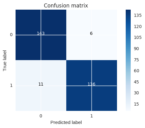
# Compute confusion matrix
cnf_matrix = confusion_matrix(y_test_undersample,y_pred_undersample)
np.set_printoptions(precision=2)
print("Recall metric in the testing dataset: ", cnf_matrix[1,1]/(cnf_matrix[1,0]+cnf_matrix[1,1]))
# Plot non-normalized confusion matrix
class_names = [0,1]
plt.figure()
plot_confusion_matrix(cnf_matrix
, classes=class_names
, title='Confusion matrix')
plt.show()
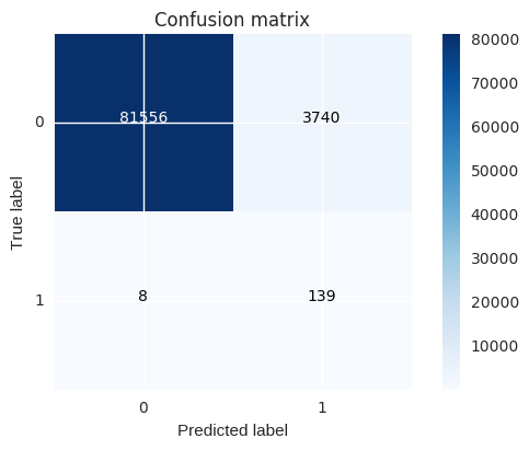
# Use this C_parameter to build the final model with the whole training dataset and predict the classes in the test
# dataset
lr = LogisticRegression(C = best_c, penalty = 'l1')
lr.fit(X_train_undersample,y_train_undersample.values.ravel())
y_pred = lr.predict(X_test.values)
# Compute confusion matrix
cnf_matrix = confusion_matrix(y_test,y_pred)
np.set_printoptions(precision=2)
print("Recall metric in the testing dataset: ", cnf_matrix[1,1]/(cnf_matrix[1,0]+cnf_matrix[1,1]))
# Plot non-normalized confusion matrix
class_names = [0,1]
plt.figure()
plot_confusion_matrix(cnf_matrix
, classes=class_names
, title='Confusion matrix')
plt.show()
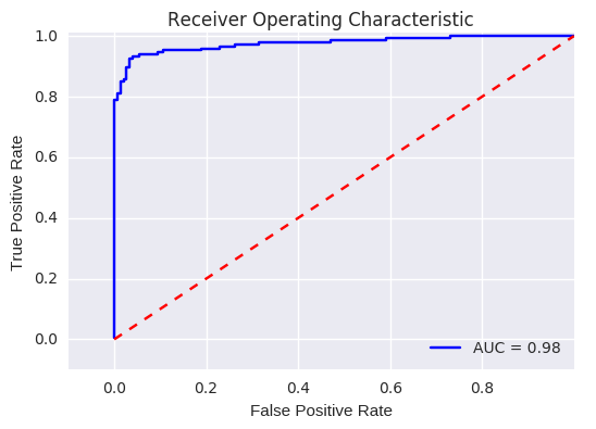
# ROC CURVE
lr = LogisticRegression(C = best_c, penalty = 'l1')
y_pred_undersample_score = lr.fit(X_train_undersample,y_train_undersample.values.ravel()).decision_function(X_test_undersample.values)
fpr, tpr, thresholds = roc_curve(y_test_undersample.values.ravel(),y_pred_undersample_score)
roc_auc = auc(fpr,tpr)
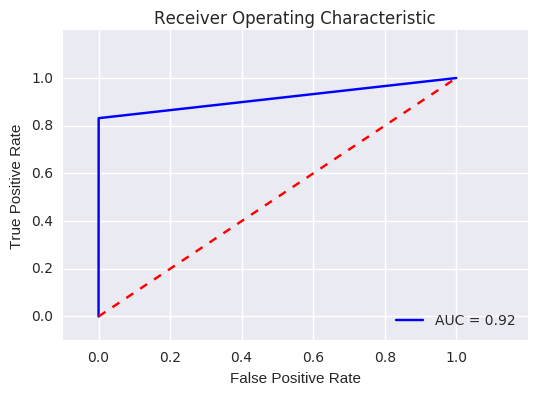
# Plot ROC
plt.title('Receiver Operating Characteristic')
plt.plot(fpr, tpr, 'b',label='AUC = %0.2f'% roc_auc)
plt.legend(loc='lower right')
plt.plot([0,1],[0,1],'r--')
plt.xlim([-0.1,1.0])
plt.ylim([-0.1,1.01])
plt.ylabel('True Positive Rate')
plt.xlabel('False Positive Rate')
plt.show()
Recall metric in the testing dataset: 0.925170068027
Recall metric in the testing dataset: 0.945578231293
Logistic regression classifier - Skewed data Having tested our previous approach, I find really interesting to test the same process on the skewed data. Our intuition is that skewness will introduce issues difficult to capture, and therefore, provide a less effective algorithm. To be fair, taking into account the fact that the train and test datasets are substantially bigger than the undersampled ones, I believe a K-fold cross validation is necessary. I guess that by splitting the data with 60% in training set, 20% cross validation and 20% test should be enough… but let’s take the same approach as before (no harm on this, it’s just that K-fold is computationally more expensive)
best_c = printing_Kfold_scores(X_train,y_train)
-------------------------------------------
C parameter:  0.01
-------------------------------------------

Iteration  1 : recall score =  0.492537313433
Iteration  2 : recall score =  0.575342465753
Iteration  3 : recall score =  0.616666666667
Iteration  4 : recall score =  0.553846153846
Iteration  5 : recall score =  0.4375

Mean recall score  0.53517851994

-------------------------------------------
C parameter:  0.1
-------------------------------------------

Iteration  1 : recall score =  0.582089552239
Iteration  2 : recall score =  0.630136986301
Iteration  3 : recall score =  0.683333333333
Iteration  4 : recall score =  0.584615384615
Iteration  5 : recall score =  0.5125

Mean recall score  0.598535051298

-------------------------------------------
C parameter:  1
-------------------------------------------

Iteration  1 : recall score =  0.55223880597
Iteration  2 : recall score =  0.630136986301
Iteration  3 : recall score =  0.733333333333
Iteration  4 : recall score =  0.615384615385
Iteration  5 : recall score =  0.5625

Mean recall score  0.618718748198

-------------------------------------------
C parameter:  10
-------------------------------------------

Iteration  1 : recall score =  0.567164179104
Iteration  2 : recall score =  0.630136986301
Iteration  3 : recall score =  0.733333333333
Iteration  4 : recall score =  0.615384615385
Iteration  5 : recall score =  0.575

Mean recall score  0.624203822825

-------------------------------------------
C parameter:  100
-------------------------------------------

Iteration  1 : recall score =  0.55223880597
Iteration  2 : recall score =  0.630136986301
Iteration  3 : recall score =  0.733333333333
Iteration  4 : recall score =  0.615384615385
Iteration  5 : recall score =  0.5625

Mean recall score  0.618718748198

*********************************************************************************
Best model to choose from cross validation is with C parameter =  10.0
*********************************************************************************
Before continuing… changing classification threshold. We have seen that by undersampling the data, our algorithm does a much better job at detecting fraud. I wanted also to show how can we tweak our final classification by changing the threshold. Initially, you build the classification model and then you predict unseen data using it. We previously used the “predict()” method to decided whether a record should belong to “1” or “0”. There is another method “predict_proba()”. This method returns the probabilities for each class. The idea is that by changing the threshold to assign a record to class 1, we can control precision and recall.
lr = LogisticRegression(C = 0.01, penalty = 'l1')
lr.fit(X_train_undersample,y_train_undersample.values.ravel())
y_pred_undersample_proba = lr.predict_proba(X_test_undersample.values)

thresholds = [0.1,0.2,0.3,0.4,0.5,0.6,0.7,0.8,0.9]

plt.figure(figsize=(10,10))

j = 1
for i in thresholds:
    y_test_predictions_high_recall = y_pred_undersample_proba[:,1] > i

    plt.subplot(3,3,j)
    j += 1

    # Compute confusion matrix
    cnf_matrix = confusion_matrix(y_test_undersample,y_test_predictions_high_recall)
    np.set_printoptions(precision=2)

    print("Recall metric in the testing dataset: ", cnf_matrix[1,1]/(cnf_matrix[1,0]+cnf_matrix[1,1]))

    # Plot non-normalized confusion matrix
    class_names = [0,1]
    plot_confusion_matrix(cnf_matrix
                          , classes=class_names
                          , title='Threshold >= %s'%i)
Recall metric in the testing dataset:  0.986394557823
Recall metric in the testing dataset:  0.952380952381
Recall metric in the testing dataset:  0.938775510204
Recall metric in the testing dataset:  0.877551020408
Recall metric in the testing dataset:  0.863945578231
Recall metric in the testing dataset:  0.823129251701
Recall metric in the testing dataset:  0.768707482993
Recall metric in the testing dataset:  0.721088435374
Recall metric in the testing dataset:  0.591836734694
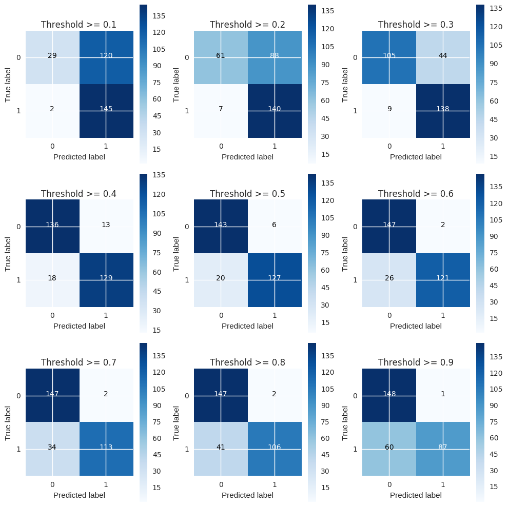
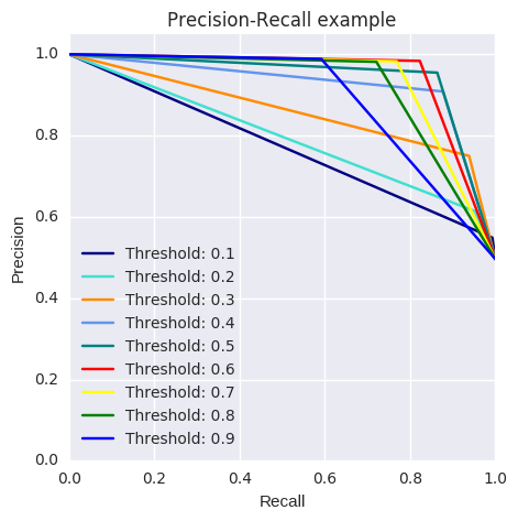
The pattern is very clear: the more you lower the required probability to put a certain in the class “1” category, more records will be put in that bucket.¶ This implies an increase in recall (we want all the “1”s), but at the same time, a decrease in precision (we misclassify many of the other class). Therefore, even though recall is our goal metric (do not miss a fraud transaction), we also want to keep the model being accurate as a whole. There is an option I think could be quite interesting to tackle this. We could assing cost to misclassifications, but being interested in classifying “1s” correctly, the cost for misclassifying “1s” should be bigger than “0” misclassifications. After that, the algorithm would select the threshold which minimises the total cost. A drawback I see is that we have to manually select the weight of each cost… therefore, I will leave this know as a thought. Going back to the threshold changing, there is an option which is the Precisio-Recall curve. By visually seeing the performance of the model depending on the threshold we choose, we can investigate a sweet spot where recall is high enough whilst keeping a high precision value.
from itertools import cycle

lr = LogisticRegression(C = 0.01, penalty = 'l1')
lr.fit(X_train_undersample,y_train_undersample.values.ravel())
y_pred_undersample_proba = lr.predict_proba(X_test_undersample.values)

thresholds = [0.1,0.2,0.3,0.4,0.5,0.6,0.7,0.8,0.9]
colors = cycle(['navy', 'turquoise', 'darkorange', 'cornflowerblue', 'teal', 'red', 'yellow', 'green', 'blue','black'])

plt.figure(figsize=(5,5))

j = 1
for i,color in zip(thresholds,colors):
    y_test_predictions_prob = y_pred_undersample_proba[:,1] > i

    precision, recall, thresholds = precision_recall_curve(y_test_undersample,y_test_predictions_prob)

    # Plot Precision-Recall curve
    plt.plot(recall, precision, color=color,
                 label='Threshold: %s'%i)
    plt.xlabel('Recall')
    plt.ylabel('Precision')
    plt.ylim([0.0, 1.05])
    plt.xlim([0.0, 1.0])
    plt.title('Precision-Recall example')
    plt.legend(loc="lower left")
What about with tensorflow
# coding: utf-8

# # Predicting Credit Card Fraud

# The goal for this analysis is to predict credit card fraud in the transactional data. I will be using tensorflow to build the predictive model, and t-SNE to visualize the dataset in two dimensions at the end of this analysis. If you would like to learn more about the data, visit: https://www.kaggle.com/dalpozz/creditcardfraud.
#
# The sections of this analysis include:
#
#  - Exploring the Data
#  - Building the Neural Network
#  - Visualizing the Data with t-SNE.

# In[ ]:

import pandas as pd
import numpy as np
import tensorflow as tf
from sklearn.cross_validation import train_test_split
import matplotlib.pyplot as plt
from sklearn.utils import shuffle
from sklearn.metrics import confusion_matrix
import seaborn as sns
import matplotlib.gridspec as gridspec
from sklearn.preprocessing import StandardScaler
from sklearn.manifold import TSNE
# In[ ]:
df = pd.read_csv("creditcard.csv")
# ## Exploring the Data
# In[ ]:
df.head()
# The data is mostly transformed from its original form, for confidentiality reasons.
# In[ ]:
df.describe()
# In[ ]:
df.isnull().sum()
# No missing values, that makes things a little easier.
#
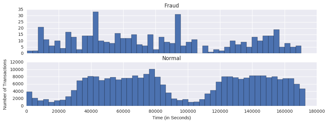
# Let's see how time compares across fraudulent and normal transactions.
# In[ ]:
print ("Fraud")
print (df.Time[df.Class == 1].describe())
print ()
print ("Normal")
print (df.Time[df.Class == 0].describe())
# In[ ]:
f, (ax1, ax2) = plt.subplots(2, 1, sharex=True, figsize=(12,4))
bins = 50
ax1.hist(df.Time[df.Class == 1], bins = bins)
ax1.set_title('Fraud')
ax2.hist(df.Time[df.Class == 0], bins = bins)
ax2.set_title('Normal')
plt.xlabel('Time (in Seconds)')
plt.ylabel('Number of Transactions')
plt.show()
# The 'Time' feature looks pretty similar across both types of transactions. You could argue that fraudulent transactions are more uniformly distributed, while normal transactions have a cyclical distribution. This could make it easier to detect a fraudulent transaction during at an 'off-peak' time.
#
# Now let's see if the transaction amount differs between the two types.
# In[ ]:
print ("Fraud")
print (df.Amount[df.Class == 1].describe())
print ()
print ("Normal")
print (df.Amount[df.Class == 0].describe())
# In[ ]:
f, (ax1, ax2) = plt.subplots(2, 1, sharex=True, figsize=(12,4))
bins = 30
ax1.hist(df.Amount[df.Class == 1], bins = bins)
ax1.set_title('Fraud')
ax2.hist(df.Amount[df.Class == 0], bins = bins)
ax2.set_title('Normal')
plt.xlabel('Amount ($)')
plt.ylabel('Number of Transactions')
plt.yscale('log')
plt.show()
# In[ ]:
df['Amount_max_fraud'] = 1
df.loc[df.Amount <= 2125.87, 'Amount_max_fraud'] = 0
# Most transactions are small amounts, less than $100. Fraudulent transactions have a maximum value far less than normal transactions, $2,125.87 vs $25,691.16.
#
# Let's compare Time with Amount and see if we can learn anything new.
# In[ ]:
f, (ax1, ax2) = plt.subplots(2, 1, sharex=True, figsize=(12,6))
ax1.scatter(df.Time[df.Class == 1], df.Amount[df.Class == 1])
ax1.set_title('Fraud')
ax2.scatter(df.Time[df.Class == 0], df.Amount[df.Class == 0])
ax2.set_title('Normal')
plt.xlabel('Time (in Seconds)')
plt.ylabel('Amount')
plt.show()
# Nothing too useful here.
#
# Next, let's take a look at the anonymized features.
# In[ ]:
#Select only the anonymized features.
v_features = df.ix[:,1:29].columns
# In[ ]:
plt.figure(figsize=(12,28*4))
gs = gridspec.GridSpec(28, 1)
for i, cn in enumerate(df[v_features]):
ax = plt.subplot(gs[i])
sns.distplot(df[cn][df.Class == 1], bins=50)
sns.distplot(df[cn][df.Class == 0], bins=50)
ax.set_xlabel('')
ax.set_title('histogram of feature: ' + str(cn))
plt.show()
# In[ ]:
#Drop all of the features that have very similar distributions between the two types of transactions.
df = df.drop(['V28','V27','V26','V25','V24','V23','V22','V20','V15','V13','V8'], axis =1)
# In[ ]:
#Based on the plots above, these features are created to identify values where fraudulent transaction are more common.
df['V1_'] = df.V1.map(lambda x: 1 if x < -3 else 0)
df['V2_'] = df.V2.map(lambda x: 1 if x > 2.5 else 0)
df['V3_'] = df.V3.map(lambda x: 1 if x < -4 else 0)
df['V4_'] = df.V4.map(lambda x: 1 if x > 2.5 else 0)
df['V5_'] = df.V5.map(lambda x: 1 if x < -4.5 else 0)
df['V6_'] = df.V6.map(lambda x: 1 if x < -2.5 else 0)
df['V7_'] = df.V7.map(lambda x: 1 if x < -3 else 0)
df['V9_'] = df.V9.map(lambda x: 1 if x < -2 else 0)
df['V10_'] = df.V10.map(lambda x: 1 if x < -2.5 else 0)
df['V11_'] = df.V11.map(lambda x: 1 if x > 2 else 0)
df['V12_'] = df.V12.map(lambda x: 1 if x < -2 else 0)
df['V14_'] = df.V14.map(lambda x: 1 if x < -2.5 else 0)
df['V16_'] = df.V16.map(lambda x: 1 if x < -2 else 0)
df['V17_'] = df.V17.map(lambda x: 1 if x < -2 else 0)
df['V18_'] = df.V18.map(lambda x: 1 if x < -2 else 0)
df['V19_'] = df.V19.map(lambda x: 1 if x > 1.5 else 0)
df['V21_'] = df.V21.map(lambda x: 1 if x > 0.6 else 0)
# In[ ]:
#Create a new feature for normal (non-fraudulent) transactions.
df.loc[df.Class == 0, 'Normal'] = 1
df.loc[df.Class == 1, 'Normal'] = 0
# In[ ]:
#Rename 'Class' to 'Fraud'.
df = df.rename(columns={'Class': 'Fraud'})
# In[ ]:
#492 fraudulent transactions, 284,315 normal transactions.
#0.172% of transactions were fraud.
print(df.Normal.value_counts())
print()
print(df.Fraud.value_counts())
# In[ ]:
pd.set_option("display.max_columns",101)
df.head()
# In[ ]:
#Create dataframes of only Fraud and Normal transactions.
Fraud = df[df.Fraud == 1]
Normal = df[df.Normal == 1]
# In[ ]:
#Set X_train equal to 75% of the fraudulent transactions.
X_train = Fraud.sample(frac=0.75)
count_Frauds = len(X_train)
#Add 75% of the normal transactions to X_train.
X_train = pd.concat([X_train, Normal.sample(frac = 0.75)], axis = 0)
#X_test contains all the transaction not in X_train.
X_test = df.loc[~df.index.isin(X_train.index)]
# In[ ]:
#Shuffle the dataframes so that the training is done in a random order.
X_train = shuffle(X_train)
X_test = shuffle(X_test)
# In[ ]:
#Add our target features to y_train and y_test.
y_train = X_train.Fraud
y_train = pd.concat([y_train, X_train.Normal], axis=1)
y_test = X_test.Fraud
y_test = pd.concat([y_test, X_test.Normal], axis=1)
# In[ ]:
#Drop target features from X_train and X_test.
X_train = X_train.drop(['Fraud','Normal'], axis = 1)
X_test = X_test.drop(['Fraud','Normal'], axis = 1)
# In[ ]:
#Check to ensure all of the training/testing dataframes are of the correct length
print(len(X_train))
print(len(y_train))
print(len(X_test))
print(len(y_test))
# In[ ]:
'''
Due to the imbalance in the data, ratio will act as an equal weighting system for our model.
By dividing the number of transactions by those that are fraudulent, ratio will equal the value that when multiplied
by the number of fraudulent transactions will equal the number of normal transaction.
Simply put: # of fraud * ratio = # of normal
'''
ratio = len(X_train)/count_Frauds
y_train.Fraud *= ratio
y_test.Fraud *= ratio
# In[ ]:
#Names of all of the features in X_train.
features = X_train.columns.values
#Transform each feature in features so that it has a mean of 0 and standard deviation of 1;
#this helps with training the neural network.
for feature in features:
mean, std = df[feature].mean(), df[feature].std()
X_train.loc[:, feature] = (X_train[feature] - mean) / std
X_test.loc[:, feature] = (X_test[feature] - mean) / std
# ## Train the Neural Net
# In[ ]:
inputX = X_train.as_matrix()
inputY = y_train.as_matrix()
inputX_test = X_test.as_matrix()
inputY_test = y_test.as_matrix()
# In[ ]:
#Number of input nodes.
input_nodes = 37
#Multiplier maintains a fixed ratio of nodes between each layer.
mulitplier = 1.5
#Number of nodes in each hidden layer
hidden_nodes1 = 15
hidden_nodes2 = round(hidden_nodes1 * mulitplier)
hidden_nodes3 = round(hidden_nodes2 * mulitplier)
#Percent of nodes to keep during dropout.
pkeep = 0.9
# In[ ]:
#input
x = tf.placeholder(tf.float32, [None, input_nodes])
#layer 1
W1 = tf.Variable(tf.truncated_normal([input_nodes, hidden_nodes1], stddev = 0.1))
b1 = tf.Variable(tf.zeros([hidden_nodes1]))
y1 = tf.nn.sigmoid(tf.matmul(x, W1) + b1)
#layer 2
W2 = tf.Variable(tf.truncated_normal([hidden_nodes1, hidden_nodes2], stddev = 0.1))
b2 = tf.Variable(tf.zeros([hidden_nodes2]))
y2 = tf.nn.sigmoid(tf.matmul(y1, W2) + b2)
#layer 3
W3 = tf.Variable(tf.truncated_normal([hidden_nodes2, hidden_nodes3], stddev = 0.1))
b3 = tf.Variable(tf.zeros([hidden_nodes3]))
y3 = tf.nn.sigmoid(tf.matmul(y2, W3) + b3)
y3 = tf.nn.dropout(y3, pkeep)
#layer 4
W4 = tf.Variable(tf.truncated_normal([hidden_nodes3, 2], stddev = 0.1))
b4 = tf.Variable(tf.zeros([2]))
y4 = tf.nn.softmax(tf.matmul(y3, W4) + b4)
#output
y = y4
y_ = tf.placeholder(tf.float32, [None, 2])
# In[ ]:
#Parameters
training_epochs = 2 #should be 2000, but the kernels dies from running for more than 1200 seconds.
display_step = 50
n_samples = y_train.size
batch = tf.Variable(0)
learning_rate = tf.train.exponential_decay(
0.01, #Base learning rate.
batch, #Current index into the dataset.
len(inputX), #Decay step.
0.95, #Decay rate.
staircase=False)
# In[ ]:
#Cost function: Cross Entropy
cost = -tf.reduce_sum(y_ * tf.log(y))
#We will optimize our model via AdamOptimizer
optimizer = tf.train.AdamOptimizer(learning_rate).minimize(cost)
#Correct prediction if the most likely value (Fraud or Normal) from softmax equals the target value.
correct_prediction = tf.equal(tf.argmax(y,1), tf.argmax(y_,1))
accuracy = tf.reduce_mean(tf.cast(correct_prediction, tf.float32))
# In[ ]:
#Initialize variables and tensorflow session
init = tf.initialize_all_variables()
sess = tf.Session()
sess.run(init)
# In[ ]:
accuracy_summary = [] #Record accuracy values for plot
cost_summary = [] #Record cost values for plot
for i in range(training_epochs):
sess.run([optimizer], feed_dict={x: inputX, y_: inputY})
# Display logs per epoch step
if (i) % display_step == 0:
train_accuracy, newCost = sess.run([accuracy, cost], feed_dict={x: inputX, y_: inputY})
print ("Training step:", i,
"Accuracy =", "{:.5f}".format(train_accuracy),
"Cost = ", "{:.5f}".format(newCost))
accuracy_summary.append(train_accuracy)
cost_summary.append(newCost)
print()
print ("Optimization Finished!")
training_accuracy = sess.run(accuracy, feed_dict={x: inputX, y_: inputY})
print ("Training Accuracy=", training_accuracy)
print()
testing_accuracy = sess.run(accuracy, feed_dict={x: inputX_test, y_: inputY_test})
print ("Testing Accuracy=", testing_accuracy)
# In[ ]:
#Plot accuracy and cost summary
f, (ax1, ax2) = plt.subplots(2, 1, sharex=True, figsize=(10,4))
ax1.plot(accuracy_summary)
ax1.set_title('Accuracy')
ax2.plot(cost_summary)
ax2.set_title('Cost')
plt.xlabel('Epochs (x50)')
plt.show()
# To summarize the confusion matrix (if you run with 2000 epochs):
#
# Correct Fraud: 102
#
# Incorrect Fraud: 21
#
# Correct Normal: 71,005
#
# Incorrect Normal: 74
#
# Although the neural network can detect most of the fraudulent transactions (82.93%), there are still some that got away. About 0.10% of normal transactions were classified as fraudulent, which can unfortunately add up very quickly given the large number of credit card transactions that occur each minute/hour/day. Nonetheless, this models performs reasonably well and I expect that if we had more data, and if the features were not pre-transformed, we could have created new features, and built a more useful neural network.
# ## Visualizing the Data with t-SNE
# First we are going to use t-SNE with the original data, then with the data we used for training our neural network. I expect/hope that the second scatter plot will show a clearer contrast between the normal and the fraudulent transactions. If this is the case, its signals that the work done during the feature engineering stage of the analysis was beneficial to helping the neural network understand the data.
# In[ ]:
#reload the original dataset
tsne_data = pd.read_csv("creditcard.csv")
# In[ ]:
#Set df2 equal to all of the fraulent and 10,000 normal transactions.
df2 = tsne_data[tsne_data.Class == 1]
df2 = pd.concat([df2, tsne_data[tsne_data.Class == 0].sample(n = 10000)], axis = 0)
# In[ ]:
#Scale features to improve the training ability of TSNE.
standard_scaler = StandardScaler()
df2_std = standard_scaler.fit_transform(df2)
#Set y equal to the target values.
y = df2.ix[:,-1].values
# In[ ]:
tsne = TSNE(n_components=2, random_state=0)
x_test_2d = tsne.fit_transform(df2_std)
# In[ ]:
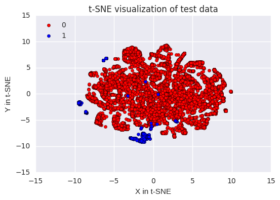
#Build the scatter plot with the two types of transactions.
color_map = {0:'red', 1:'blue'}
plt.figure()
for idx, cl in enumerate(np.unique(y)):
plt.scatter(x = x_test_2d[y==cl,0],
y = x_test_2d[y==cl,1],
c = color_map[idx],
label = cl)
plt.xlabel('X in t-SNE')
plt.ylabel('Y in t-SNE')
plt.legend(loc='upper left')
plt.title('t-SNE visualization of test data')
plt.show()
# The are two main groupings of fraudulent transactions, while the remaineder are mixed within the rest of the data.
#
# Note: I have only used 10,000 of the 284,315 normal transactions for this visualization. I would have liked to of used more, but my laptop crashes if many more than 10,000 transactions are included. With only 3.15% of the data being used, there should be some accuracy to this plot, but I am confident that the layout would look different if all of the transactions were included.
# In[ ]:
#Set df_used to the fraudulent transactions' dataset.
df_used = Fraud
#Add 10,000 normal transactions to df_used.
df_used = pd.concat([df_used, Normal.sample(n = 10000)], axis = 0)
# In[ ]:
#Scale features to improve the training ability of TSNE.
df_used_std = standard_scaler.fit_transform(df_used)
#Set y_used equal to the target values.
y_used = df_used.ix[:,-1].values
# In[ ]:
x_test_2d_used = tsne.fit_transform(df_used_std)
# In[ ]:
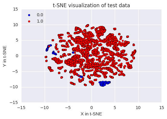
color_map = {1:'red', 0:'blue'}
plt.figure()
for idx, cl in enumerate(np.unique(y_used)):
plt.scatter(x=x_test_2d_used[y_used==cl,0],
y=x_test_2d_used[y_used==cl,1],
c=color_map[idx],
label=cl)
plt.xlabel('X in t-SNE')
plt.ylabel('Y in t-SNE')
plt.legend(loc='upper left')
plt.title('t-SNE visualization of test data')
plt.show()
# It appears that the work we did in the feature engineering stage of this analysis has been for the best. We can see that the fraudulent transactions are all part of a group of points. This suggests that it is easier for a model to identify the fraudulent transactions in the testing data, and to learn about the traits of the fraudulent transactions in the training data.
Fraud
count       492.000000
mean      80746.806911
std       47835.365138
min         406.000000
25%       41241.500000
50%       75568.500000
75%      128483.000000
max      170348.000000
Name: Time, dtype: float64

Normal
count    284315.000000
mean      94838.202258
std       47484.015786
min           0.000000
25%       54230.000000
50%       84711.000000
75%      139333.000000
max      172792.000000
Name: Time, dtype: float64
Fraud
count     492.000000
mean      122.211321
std       256.683288
min         0.000000
25%         1.000000
50%         9.250000
75%       105.890000
max      2125.870000
Name: Amount, dtype: float64

Normal
count    284315.000000
mean         88.291022
std         250.105092
min           0.000000
25%           5.650000
50%          22.000000
75%          77.050000
max       25691.160000
Name: Amount, dtype: float64
/home/dsno800/anaconda3/lib/python3.5/site-packages/statsmodels/nonparametric/kdetools.py:20: VisibleDeprecationWarning: using a non-integer number instead of an integer will result in an error in the future
  y = X[:m/2+1] + np.r_[0,X[m/2+1:],0]*1j
1.0    284314
0.0       492
Name: Normal, dtype: int64

0    284315
1       492
Name: Fraud, dtype: int64
213605
213605
71202
71202
Training step: 0 Accuracy = 0.82952 Cost =  297271.81250

Optimization Finished!
Training Accuracy= 0.98552

Testing Accuracy= 0.985548
Using SMOTE to predict
# This on is not running it has some cross-validation problems.

# coding: utf-8

# This method gives a pretty descent result with default values of the algorithms.
#
# With a test set using 20% of the full data set, we have an ROC AUC of 0.92
#
# As the data set is unbalanced, we use an oversampling method (SMOTE) to obtain a balanced set. After that, we train a Random Forest classifier

# In[ ]:

import pandas as pd
import scipy
from imblearn.over_sampling import SMOTE
from sklearn.ensemble import RandomForestClassifier
from sklearn.metrics import confusion_matrix
from sklearn.cross_validation import train_test_split

# ### Build the data set from file

# In[ ]:

credit_cards=pd.read_csv('creditcard.csv')

columns=credit_cards.columns
# The labels are in the last column ('Class'). Simply remove it to obtain features columns
features_columns=columns.delete(len(columns)-1)

features=credit_cards[features_columns]
labels=credit_cards['Class']

# ### Build train and test sets (20% of data reserved to test set)

# In[ ]:

features_train, features_test, labels_train, labels_test = train_test_split(features,
                                                                            labels,
                                                                            test_size=0.2,
                                                                            random_state=0)

# ### Create from train set a new data set to obtain a balanced data set using SMOTE

# In[ ]:

oversampler=SMOTE(random_state=0)
os_features,os_labels=oversampler.fit_sample(features_train,labels_train)

# In[ ]:

# verify new data set is balanced
len(os_labels[os_labels==1])

# ### Perform training of the random forest using the (over sampled) train set

# In[ ]:

clf=RandomForestClassifier(random_state=0)
clf.fit(os_features,os_labels)

# In[ ]:

# perform predictions on test set
actual=labels_test
predictions=clf.predict(features_test)

# ### confusion matrix on test set gives an encouraging result

# In[ ]:

confusion_matrix(actual,predictions)

# ### Let's go further and use the roc_auc indicator
#
# #### see https://datamize.wordpress.com/2015/01/24/how-to-plot-a-roc-curve-in-scikit-learn for a quick introduction

# In[ ]:

from sklearn.metrics import roc_curve, auc

false_positive_rate, true_positive_rate, thresholds = roc_curve(actual, predictions)
roc_auc = auc(false_positive_rate, true_positive_rate)
print (roc_auc)

# ### According to the previous article, this result can be considered as very good as it is between 0.9 and 1
#
# ### Let's plot a shiny curve for the final result

# In[ ]:

import matplotlib.pyplot as plt
plt.title('Receiver Operating Characteristic')
plt.plot(false_positive_rate, true_positive_rate, 'b', label='AUC = %0.2f'% roc_auc)
plt.legend(loc='lower right')
plt.plot([0,1],[0,1],'r--')
plt.xlim([-0.1,1.2])
plt.ylim([-0.1,1.2])
plt.ylabel('True Positive Rate')
plt.xlabel('False Positive Rate')

# ## Acknoledgments
#
# Many thank's to [AtherRizvi][1] and it's [notebook][2] for the informations about ROC and AUC
#
#
#   [1]: https://www.kaggle.com/ather123
#   [2]: https://www.kaggle.com/ather123/d/dalpozz/creditcardfraud/randomforestclassifier-solution/notebook/ "notebook"
0.915709683559

<matplotlib.text.Text at 0x7fbf091ca748>